Running machine learning models have become much easier in recent years. The prevalence of tutorials and model packages makes it much more convenient for people to apply various theoretically complex algorithms on their datasets and thrive. So to excel in the field of data science, one cannot simple KNOW how to use models, but also appreciate each model's significance and select proper models wisely. That's where feature selections and model selections come in. Both turn out to be challenging and extremely useful in the same time. In light of this, I want to take down the notes I learned through practice and tutorials some key aspects of these two things.
Feature Selection
Benefits
It enables the machine learning algorithm to train faster.
It reduces the complexity of a model and makes it easier to interpret.
It improves the accuracy of a model if the right subset is chosen.
It reduces Overfitting
Methods
Here we discuss about some widely used methods for feature selections. To facilitate the demo code, we require the following packages to be applied and data being tuned:
1
2
3
4
5
6
7
8
9
10
11
12
13
14
15
16
17
18
from sklearn.datasets import load_boston
import pandas as pd
import numpy as np
import matplotlib.pyplot as plt
import seaborn as sns
import statsmodels.api as sm

from sklearn.model_selection import train_test_split
from sklearn.linear_model import LinearRegression, RidgeCV, LassoCV, Ridge, Lasso
from sklearn.feature_selection import RFE

%matplotlib inline
#Loading the dataset
x = load_boston()
df = pd.DataFrame(x.data, columns = x.feature_names)
df["MEDV"] = x.target
X = df.drop("MEDV",1)   #Feature Matrix
y = df["MEDV"]          #Target Variable
Filter Methods
No mining algorithm included
Uses the exact assessment criterion which includes distance, information, dependency, and consistency.
The filter method uses the principal criteria of ranking technique and uses the rank ordering method for variable selection.
Generally used as a dasta preprocessing step
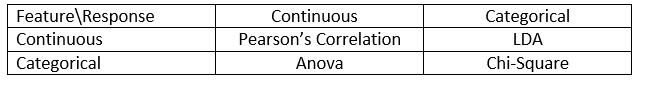
Several main filter methods based on the variable attributes: filter methods
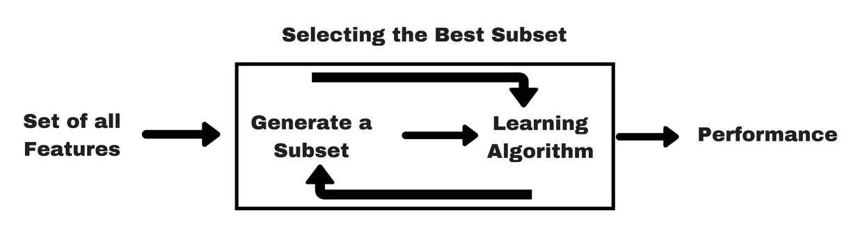
Wrapper Methods
workflow: filter methods
- Use a subset of features and train a model using them. Based on the inferences that we draw from the previous model, we decide to add or remove features from your subset
Computationally expensive
3 Types:
Forward Selection: An iterative method
Start with having no feature in the model.
In each iteration, we keep adding the feature which best improves our model till an addition of a new variable does not improve the performance of the model.
Backward Elimination: An iterative method
Start with all the features and removes the least significant feature at each iteration which improves the performance of the model.
We repeat this until no improvement is observed on removal of features.
E.g. If the p-value is above 0.05 then we remove the feature, else we keep it.
# Adding constant column of ones, mandatory for sm.OLS model
X_1 = sm.add_constant(X)
# Fitting sm.OLS model
model = sm.OLS(y,X_1).fit()
display(model.pvalues)
# Backward Elimination
cols = list(X.columns)
pmax = 1
while (len(cols)>0):
    p= []
    X_1 = X[cols]
    X_1 = sm.add_constant(X_1)
    model = sm.OLS(y,X_1).fit()
    p = pd.Series(model.pvalues.values[1:],index = cols)
    pmax = max(p)
    feature_with_p_max = p.idxmax()
    if(pmax>0.05):
        cols.remove(feature_with_p_max)
    else:
        break
selected_features_BE = cols
print(selected_features_BE)
Recursive Feature elimination: A greedy optimization algorithm
It repeatedly creates models and keeps aside the best or the worst performing feature at each iteration.
It constructs the next model with the left features until all the features are exhausted.
It then ranks the features based on the order of their elimination
1
2
3
4
5
6
7
8
9
10
11
model = LinearRegression() #Initializing RFE model rfe = RFE(model, 7) #Transforming data using RFE X_rfe = rfe.fit_transform(X,y) #Fitting the data to model model.fit(X_rfe,y) print(rfe.support_) print(rfe.ranking_) >>> [FalseFalseFalseTrueTrueTrueFalseTrueTrueFalseTrueFalseTrue] >>> [2431117115161]
Here we took LinearRegression model with 7 features and RFE gave feature ranking as above, but the selection of number '7' was random. Now we need to find the optimum number of features, for which the accuracy is the highest. We do that by using loop starting with 1 feature and going up to 13. We then take the one for which the accuracy is highest.
#no of features nof_list=np.arange(1,13) high_score=0 #Variable to store the optimum features nof=0 score_list =[] for n inrange(len(nof_list)): X_train, X_test, y_train, y_test = train_test_split(X,y, test_size = 0.3, random_state = 0) model = LinearRegression() rfe = RFE(model,nof_list[n]) X_train_rfe = rfe.fit_transform(X_train,y_train) X_test_rfe = rfe.transform(X_test) model.fit(X_train_rfe,y_train) score = model.score(X_test_rfe,y_test) score_list.append(score) if(score>high_score): high_score = score nof = nof_list[n] print("Optimum number of features: %d" %nof) print("Score with %d features: %f" % (nof, high_score))
As seen from above code, the optimum number of features is 10. We now feed 10 as number of features to RFE and get the final set of features given by RFE method
1
2
3
4
5
6
7
8
9
10
11
cols = list(X.columns)
model = LinearRegression()
#Initializing RFE model
rfe = RFE(model, 10)
#Transforming data using RFE
X_rfe = rfe.fit_transform(X,y)
#Fitting the data to model
model.fit(X_rfe,y)
temp = pd.Series(rfe.support_,index = cols)
selected_features_rfe = temp[temp==True].index
print(selected_features_rfe)
(*) Bidirectional Elimination: A combination of Forward Selection & Backword Elimination
Self-defined Methods There are many interesting methods that can be directly applied in experimentations. However, one method that caught my eyes is the Boruta method:
Boruta Method (Using shadow features and random forest)
The main reason I liked this is because its application on Random Forest and XGBoost models.
It generally works well with well structured data and relatively smaller datasets.
In the hindsight, it is still relatively slower as compared to some simpler selection criterion, and it does not handle multicollinearity immediately.
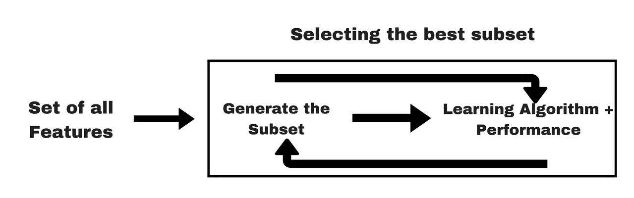
Embedded Methods It combines the qualities of filter and wrapper methods. It's implemented by algorithms that have their own built-in feature selection methods
Workflow
Embedded Method Workflow
Here in the demo code we will do feature selection using Lasso regularization. If the feature is irrelevant, lasso penalizes it's coefficient and make it 0. Hence the features with coefficient = 0 are removed and the rest are taken.
1
2
3
4
5
6
7
8
9
10
11
12
13
14
reg = LassoCV()
reg.fit(X, y)
print("Best alpha using built-in LassoCV: %f" % reg.alpha_)
print("Best score using built-in LassoCV: %f" % reg.score(X,y))
>>> Best alpha using built-in LassoCV: 0.724820
>>> Best score using built-in LassoCV: 0.702444
coef = pd.Series(reg.coef_, index = X.columns)
print("Lasso picked " + str(sum(coef != 0)) + " variables and eliminated the other " +  str(sum(coef == 0)) + " variables")
>>> Lasso picked 10 variables and eliminated the other 3 variables
imp_coef = coef.sort_values()
import matplotlib
matplotlib.rcParams['figure.figsize'] = (8.0, 10.0)
imp_coef.plot(kind = "barh")
plt.title("Feature importance using Lasso Model")
Filter vs Wrapper
Now let us make a comparison between filter methods and wrapper methods, the two most commonly used ways in feature selection.
Characteristics
Filter Method
Wrapper Methods
Measure of feature relevance
correlation with dependent variable
actually training a model on a subset of feature
Speed
Much faster
Slower due to model training
Performance Evaluation
statistical methods for evaluation
Model results cross validation
Quality of feature set selected
May be suboptimal
Guaranteed to output optimal/near-optimal feature set
Overfitting ?
Less likely
Much more prone to
Model Selection
Here we must clarify one important conceptual misunderstanding:
Note: Classical Model selection mainly focuses on performing metrics evaluations through different models, tuning the model parameter and variating the training datasets. The choice of model in the end is often manual. Hence, it differs from the automated model selection procedure where the final selection of model is also done automatically. The latter is often known as AutoML, and has gained quick wide popularity in recent years.
We now think about what are the main strategies to improve model performance:
Use a more complicated/more flexible model
Use a less complicated/less flexible model
Tuning hyperparameters
Gather more training samples
Gather more data to add features to each sample Clearly, the first 4 are model selection strategies, and the last one is feature selection.
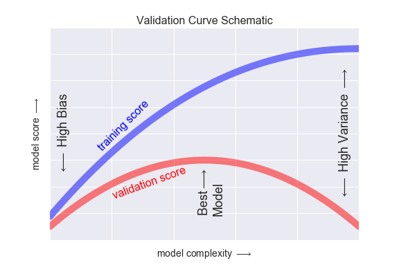
When we make these adjustments, we must keep in mind the The Bias-variance trade-off:
bias: Usually the case where the model underfits, i.e. it does not have enough model flexibility to suitably account for all the features in the data
variance: Usually the case where the model overfits, i.e. so much model flexibility that the model ends up accounting for random errors as well as the underlying data distribution
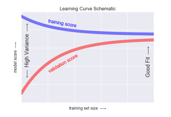
For high-bias models, the performance of the model on the validation set is similar to the performance on the training set.
For high-variance models, the performance of the model on the validation set is far worse than the performance on the training set.
We can easily visualize this via the learning curve Plot 1: The curve to find the best amount of train set size (too low –> high variance; too high –> high bias)
In the meantime, we observe from the validation curve below that model complexity/hyperparameter choices affect the model performances as well Plot 2: The curve to find the best hyperparameters
For more details on metrics evaluation and hyperparameter tuning with feedback from validation sets, interested readers can read my blogs on these topics as well.