Some Supervised Learning Models

Overview

Almost everyone who learned about data science or machine learning knows what supervised learning is. However, not many have dived deep into the details of those well-known models. In this blog, I will share some critical aspects of these models (mainly mathematical) that will become helpful in both research and practical work. One note on functionality is that these models work for both regression and classification problems.

KNN

1. Definition

• K nearest neighbors is a simple algorithm that stores all available cases and predict the numerical target based on a similarity measure (e.g., distance functions)
• Non-parametric technique
• Distance functions can be
  • Euclidean:
  • Manhattan (Or Hamming in the case of Classification):
  • Minkowski:
• Preprocessing
  • Standardized Distance: One major drawback in calculating distance measures directly from the training set is in the case where variables have different measurement scales or there is a mixture of numerical and categorical variables. The solution is to do standardization on each variable
  • Dimension Reduction: Usually KNN's speed gets much slower when number of attributes increase. Hence we need to reduce the number of dimensions using techniques such as PCA and SVD

2. Choice of K

• In general, a large K value is more precise as it reduces the overall noise; however, the compromise is that the distinct boundaries within the feature space are blurred (Lower prediction accuracy if K is too large).
• Need to use cross validation to determine an optimal K

3. Strength and Weakness

• Advantage
  • The algorithm is simple and easy to implement.
  • There's no need to build a model, tune several parameters, or make additional assumptions.
  • The algorithm is versatile. It can be used for classification, regression, and search (as we will see in the next section).
  • Good interpretability. There are exceptions: if the number of neighbors is large, the interpretability deteriorates
    • "We did not give him a loan, because he is similar to the 350 clients, of which 70 are the bad, and that is 12% higher than the average for the dataset".
• Disadvantages
  • The algorithm gets significantly slower as the number of examples and/or predictors/independent variables increase.
  • KNN doesn't know which attributes are more import ant
  • Doesn't handle missing data gracefully
  • Slow during prediction (not training)

4. Suitable scenario

• KNN is bad if you have too many data points and speed is important
• In ensemble model: k-NN is often used for the construction of meta-features (i.e. k-NN predictions as input to other models) or for stacking/blending
• When you are solving a problem which directly focusses on finding similarity between observations, K-NN does better because of its inherent nature to optimize locally (i.e: KNN-search)
• Real Life Example: a simple recommender system (e.g: Given our movies data set, what are the 5 most similar movies to a movie query)

5. Interview Questions

1. Use 1 line to describe KNN
   • Answer: KNN works by finding the distances between a query and all the examples in the data, selecting the specified number examples (K) closest to the query, then votes for the most frequent label (in the case of classification) or averages the labels (in the case of regression).

6. Simple implementations

## For Regression
from sklearn.neighbors import KNeighborsClassifier
from sklearn.neighbors import KNeighborsRegressor
from sklearn.model_selection import GridSearchCV
from sklearn.metrics import confusion_matrix,mean_squared_error,accuracy_score
from sklearn.preprocessing import MinMaxScaler
from sklearn.model_selection import train_test_split

##Randomly generate some data

data  = pd.DataFrame(np.random.randint(low = 2,high = 100,size = (1000, 4)),
                     columns=["Target","A","B","C"])
data.head()

train_x,test_x,train_y,test_y = train_test_split(data.iloc[:,1:],data.Target,test_size = 0.2)
print(train_x.shape, test_x.shape)

scaler = MinMaxScaler(feature_range=(0,1))

scaler.fit(train_x)
scaled_train_x = pd.DataFrame(scaler.transform(train_x),columns=['A','B','C'])
scaled_test_x = pd.DataFrame(scaler.transform(test_x),columns=["A","B","C"])

###Basic Performance testing
knn_regressor = KNeighborsRegressor(n_neighbors=3,algorithm="brute",weights="distance")
knn_regressor.fit(scaled_train_x, train_y)

train_pred = knn_regressor.predict(scaled_train_x)
test_pred = knn_regressor.predict(scaled_test_x)

print(mean_squared_error(train_y,train_pred))
print(mean_squared_error(test_y,test_pred))

###Grid Search to determine K
knn_regressor = KNeighborsRegressor(algorithm="brute",weights="distance")
params = {"n_neighbors": [1,3,5],"metric": ["euclidean", "cityblock"]}
grid = GridSearchCV(knn_regressor,param_grid=params,scoring="neg_mean_squared_error",cv=5)

grid.fit(scaled_train_x, train_y)
print(grid.best_params_)
print(grid.best_score_)

best_knn = grid.best_estimator_
train_pred = best_knn.predict(scaled_train_x)
test_pred = best_knn.predict(scaled_test_x)

SVM

1. Definition

• Normally a binary classification
• Basic Ideology: SVM is based on the idea of finding a hyperplane that best separates the features into different domains.
• Both for Regression and classification
  • SVR
  • SVC
• Support vectors: The points closest to the hyperplane
• margin maximizing hyperplane: the bound that maximize the distances from support vectors
• hard margin SVM: If the points are linearly separable then only our hyperplane is able to distinguish between them. Then we have very strict constraints to correctly classify each and every datapoint
• Soft margin SVM: If the points are not linearly separable then we need an update so that our function may skip few outliers and be able to classify almost linearly separable points. For this reason, we introduce a new Slack variable(ξ)
  • We use CV to determine whether allowing certain amount of misclassification results in better classification in the long run
• Kernel: used to systematically find the specfic transformation that leads to class separation
  1. Polynomial Kernel: where = constant term and = degree of kernel
     • done via Dot Product of a Feature Engineered Matrix
  2. Radial basis function kernel (RBF)/ Gaussian Kernel: where = Euclidean distance between &
     • γ: As the value of increases the model gets overfits. As the value of decreases the model underfits
     • For Gaussian kernel:
• Most Important Idea abut Kernel: Our powerful kernel function actually calculate the high-dimensional relationships WITHOUT actually transforming the data to higher dimensions
• Multiclass classification:
  • 2 types of strategy
    • One vs. All: N-class instances then N binary classifier models, then pick the prediction of a non-zero class which is the most certain.

      

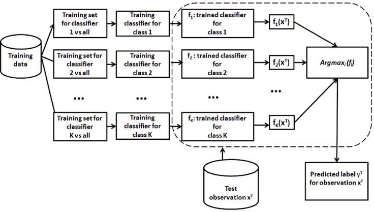
      One-vs-Rest classification

    • One vs. One: N-class instances then N* (N-1)/2 binary classifier models (adopted in SVM). At prediction time, a voting scheme is applied: all C(C−1)/2 classifiers are applied to an unseen sample and the class that got the highest number of "+1" predictions gets predicted by the combined classifier.
  • decision_function_shape='ovo' in the parameter to specify one-vs-one, else default is ovr

2. Pros & Cons

Pros

• It is really effective in the higher dimension.
• Its solution is global optimal
• Effective when the number of features are more than training examples.
• Great when the data is noise-free and separable
• Less affected by outliers (if they are not the support vectors)
• SVM is suited for extreme case binary classification.

Cons

• For larger dataset, it requires a large amount of time to process.
• Does not perform well in case of overlapped classes
• Cannot handle categorical data must convert via proper encoding
• Selection of hyperparameter/Kernel can be difficult
• resulting boundary plane are very difficult to interpret

3. Application

• When you need a non-linear approximator, use it
• When your dataset has a lot of features, use it
• When the matrix is sparse, use it
• When the data is unstructured, it is not used

4. Simple Implementation

from sklearn.svm import SVC

svc=SVC(kernel='linear') # Choices include 'rbf', 'poly', 'sigmoid'
svc.fit(X_train,y_train)
y_pred=svc.predict(X_test)
print('Accuracy Score:')
print(metrics.accuracy_score(y_test,y_pred))

Decision Tree

1. Definition

• Decision Tree is a tree-based model that predict the class or value of the target variable by learning simple decision rules inferred from prior data(training data).
• use a layered splitting process, where at each layer they try to split the data into two or more groups, so that data that fall into the same group are most similar to each other (homogeneity), and groups are as different as possible from each other (heterogeneity).
• It apples a top-down approach to data, so that given a data set, DTs try to group and label observations that are similar between them, and look for the best rules that split the observations that are dissimilar between them until they reach certain degree of similarity.
• Non-parametric technique
• Pruning: a technique used to deal with overfitting, that reduces the size of DTs by removing sections of the Tree that provide little predictive or classification power. Simpler trees prefered (according to Occam's Razor)
  • Post-prune: When you take a fully grown DT and then remove leaf nodes only if it results in a better model performance. This way, you stop removing nodes when no further improvements can be made.

2. Types of DT

1. CHAID (Chi-squared Automatic Interaction Detection)
   • multiway DT
   • chooses the independent variable that has the strongest interaction with the dependent variable.
   • The selection criteria:
     1. For regression: F-test
     2. For classification: chi-square test
   • Has no pruning function
2. CART (Classification And Regression Tree)
   • binary DT
   • handles data in its raw form (no preprocessing needed),
   • can use the same variables more than once in different parts of the same DT, which may uncover complex interdependencies between sets of variables.
   • The selection metric:
     1. For Classification: Gini Impurity Index
        • where is the % of data with label in the split
        • The lower value indicates a better spliting
     2. For Regression: Least Square Deviation (LSD)
        • the sum of the squared distances (or deviations) between the observed values and the predicted values.
        • Often refered as 'sqaured residual', lower LSD means better split
   • doesn't use an internal performance measure for Tree selection/testing
3. Iterative Dichotomiser 3 (ID3)
   • classification DT
   • Entropy:
     • Single Attribute:
     • Multiple Attribute: where → Current state and → Selected attribute
     • The higher the entropy, the harder it is to draw any conclusions from that information.
   • Follows the rule — A branch with an entropy of zero is a leaf node and A brach with entropy more than zero needs further splitting
   • The selection metric:
     • Information Gain: where is number of splits and is a particular split
     • The higher the gain, the better the split
   • Limitation: it can't handle numeric attributes nor missing values
4. C4.5
   • The successor of ID3 and represents an improvement in several aspects
     • can handle both continuous and categorical data (regression + classification)
     • can deal with missing values by ignoring instances that include non-existing data
   • The selection metric:
     • Gain ratio: a modification of Information gain that reduces its bias and is usually the best option
   • Windowing: the algorithm randomly selects a subset of the training data (called a "window") and builds a DT from that selection.
     • This DT is then used to classify the remaining training data, and if it performs a correct classification, the DT is finished. Otherwise, all the misclassified data points are added to the windows, and the cycle repeats until every instance in the training set is correctly classified by the current DT.
     • It captures all the "rare" instances together with sufficient "ordinary" cases.
   • Can be pruned: pruning method is based on estimating the error rate of every internal node, and replacing it with a leaf node if the estimated error of the leaf is lower.

3. Strength and Weakness

• Advantage
  • The algorithm is simple and easy to implement.
  • Require very little data preparation
  • The cost of using the tree for inference is logarithmic in the number of data points used to train the tree. Hence the training speed is high
  • Good interpretability.
• Disadvantages
  • Overfitting is quite common with decision trees simply due to the nature of their training. It's often recommended to perform some type of dimensionality reduction such as PCA so that the tree doesn't have to learn splits on so many features
  • high variance, which means that a small change in the data can result in a very different set of splits, making interpretation somewhat complex.
  • vulnerable to becoming biased to the classes that have a majority in the dataset. It's always a good idea to do some kind of class balancing such as class weights, sampling, or a specialised loss function.
  • In more technical terms: it always look for a greedy option to split, thus more inclined towards a locally optimal split instead of a gloablly optimal one

4. Suitable scenario

Consideration:

• If the goal is better predictions, we should prefer RF, to reduce the variance.
• If the goal is exploratory analysis, we should prefer a single DT , as to understand the data relationship in a tree hierarchy structure.
• If there is a high non-linearity & complex relationship between dependent & independent variables, a tree model will outperform a classical regression method.
• When computational power is low, DT should be used
• When important features in the attributes are already identified, DT can be used
• When you demand more interpretability, DT should be used
  

Use cases:

• healthcare industry: the screening of positive cases in the early detection of cognitive impairment
• Environment/Agriculture: DTs are used in agriculture to classify different crop types and identify their phenological stages/recognize different causes of forest loss from satellite imagery
• Sentiment Analysis: identify emotion from text
• Finance: Fraud Detection

5. Simple implementations

from sklearn import tree
dt = tree.DecisionTreeClassifier(random_state=1, max_depth=4)
dt.fit(data_train, label_train)
dt_score_train = dt.score(data_train, label_train)  
print("Training score: ",dt_score_train)
dt_score_test = dt.score(data_test, label_test)
print("Testing score: ",dt_score_test)

dt2.predict(data_pred)

Naive Bayes

1. Definition

• The Naïve Bayes Classifier belongs to the family of probability classifier, using Bayesian theorem. The reason why it is called 'Naïve' because it requires rigid independence assumption between input variables.
• The classification formula is simple:
• Why is it called 'Naive': It is naive because while it uses conditional probability to make classifications, the algorithm simply assumes that all features of a class are independent. This is considered naive because, in reality, it is not often the case.
• Laplace Smoothing is also applied in some cases to solve the problem of zero probability.
• Different types of NB:
  • Gaussian: It is used in classification and it assumes that features follow a normal distribution.
  • Multinomial: It is used for discrete counts. For example, let's say, we have a text classification problem. Here we can consider Bernoulli trials which is one step further and instead of 'word occurring in the document', we have 'count how often word occurs in the document', you can think of it as 'number of times outcome number x_i is observed over the n trials'.
  • Bernoulli: The binomial model is useful if your feature vectors are binary (i.e. zeros and ones). One application would be text classification with 'bag of words' model where the 1s & 0s are 'word occurs in the document' and 'word does not occur in the document' respectively.
• You might think to apply some classifier combination technique like ensembling, bagging and boosting but these methods would not help. Actually, "ensembling, boosting, bagging" won't help since their purpose is to reduce variance. Naive Bayes has no variance to minimize.

2. Pros & Cons

Pros

• It is easy and fast to predict the class of the test data set. It also performs well in multi-class prediction.
• When assumption of independence holds, a Naive Bayes classifier performs better compare to other models like logistic regression and you need less training data.
• It perform well in case of categorical input variables compared to numerical variable(s). For numerical variable, normal distribution is assumed (bell curve, which is a strong assumption).

Cons

• Can't learn the relationship among the features because assumes feature independence
• the assumption of independent predictors unlikely to hold. In real life, it is almost impossible that we get a set of predictors which are completely independent.

3. Applications

• Realtime prediction (because it's fast)
• When Dataset is Huge (high-dimension)
• When training dataset is small
• Text classification/ Spam Filtering/ Sentiment Analysis: Naive Bayes classifiers mostly used in text classification (due to better result in multi class problems and independence rule) have higher success rate as compared to other algorithms. As a result, it is widely used in Spam filtering (identify spam e-mail) and Sentiment Analysis (in social media analysis, to identify positive and negative customer sentiments)
• Recommendation System: Naive Bayes Classifier and Collaborative Filtering together builds a Recommendation System that uses machine learning and data mining techniques to filter unseen information and predict whether a user would like a given resource or not.

4. Simple Implementation

from sklearn.naive_bayes import GaussianNB
model = GaussianNB()

# fit the model with the training data
model.fit(train_x,train_y)

# predict the target on the train dataset
predict_train = model.predict(train_x)
print('Target on train data',predict_train)