Hyperparameter Tuning

Overview

Hyperparameter tuning is a large field of study, just like any subjects under the topic of machine learning. In fact, I really need to thank this topic for bringing me into the field of Bayesian Optimization and Bandit, as well as the future sequential decision-making models I researched on. In this blog, I'll present some classical and popular methods for hyperparameter tuning. Before that, let us make crystal clear what is hyperparameter and why is it so important.

Hyperparameter vs parameter

• Parameters: The variables inside the model that are gradually updated and estimated via data training. For example, the coefficients in a regression model, or the weights of a deep neural network.
• hyperparameters: The input variables to a model that stay the same during the training. They are often used in the algorithm to actually help estimate the model parameters. For example, the error rate specified in a statistical learning model like Support Vector Machine or the learning rate in deep neural networks.

From the description above, we see that we should choose our hyperparameters wisely so that the parameters which helps our model stand out from the rest models using the same algorithm. Unfortunately, these inputs to the models are often in a continuous space, and we will rarely be able to explore every possible value. That's why numerous tuning methods were devised to help us obtain good hyperparameters that improve our models' performances.

Automated hyperparameter tuning

Although the job can be via manual selection. This is a very tedious process. Instead, many algorithms surfaced to help us overcome this difficulty.

1. Random Search

In each iteration, we choose from the input space (for hyperparameters) random combination of hyperparameters to run the model. After our budget for iterations runs out, we then compare the performance of model with each combination and select the best one.

2. Grid Search

As compared to random search, we choose from the input space a set of hyperparameters combinations evenly (sometimes with additional greedy exploration). We then choose from the observed models the best one. This avoid unintential negligence of certain regions in the input space.

Unfortunately, the two methods above require the “boundedness” assumption for the input domain. The following methods allow for a general open set for the input spaces.

3. Bayesian Optimization

In general, a sequential design strategy for global extrema computation of black-box functions that does not assume any functional form. It can be applied in hyperparameter optimization as well.

• Strategy Description:
  • Prior: a function that is applied on existing observations. The prior captures the bellief about the behaviour of the function.
  • Posterior: the distribution function over the objective function after the priors are evaluated on the observations.
  • Acquisition function: the functions to determine the next query point based on the optimization objective
• Methods to define the prior/posterior distributions:
  1. Gaussian Process
     • Finding the values of p(y|x) where y is the function to be minimized (e.g., validation loss) and x is the value of hyperparameter
     • More expensive
     • Usually executed with few observations
     • Assume Gaussian distribution initially
     • Generate new points (expected value and variance) with in the support
  2. Tree of Parzen Estimator
     • Less expensive
     • construct 2 distributions for 'high' and 'low' points, and then finds the location tht maximizes the expected improvement of 'low' points
     • models P(x|y) and P(y)
     • The drawback is the lack of interaction between hyperparameters.
• Acquisition Functions:
  • Mainly trade-off exploitation and exploration so as to minimize the number of function queries
  • Exploitation means sampling where the surrogate model predicts a high objective
  • Exploration means sampling at locations where the prediction uncertainty is high.
  • Several types of functions:
    • Probability of improvement
    • Expected improvement
    • Upper Confidience Bound
    • Thompson Sampling
    • Entropy Search Methods
  • Optimization of functions:
    • Mainly through discretization using Newton's Method such as lbfgs

In general, BO is widely applied in hyperparameter optimization, and is often ideal when the function evaluation is very costly, as its convergence rate is often much better as compared to other methods.

4. Hyperband

Hyperband is a variation of random search, but with the decision-making models from bandit algorithms to help find the best time allocation for each of the configurations. The method is theoretically sound, and has great variants ASHA (Asynchronous Hyperband) and BOHB (Bayesian Optimization with Hyperband) This also aroused my interests in bandit problems. You may read the research paper here.

Genetic Algorithm

1. Definition

• A search heuristic that is inspired by Charles Darwin’s theory of natural evolution.
• This algorithm reflects the process of natural selection where the fittest individuals are selected for reproduction in order to produce offspring of the next generation.
• 5 phases:

  

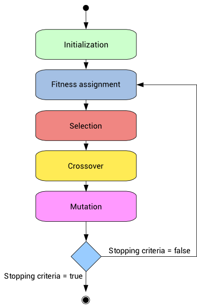
  Genetic Algorithm Procedure

  • Initial population
    • stochastic process: the individuals' genes are usually initialized at random.
  • Fitness function
    • Determines the ability (Fitness score) of an individual to compete with other individuals)
    • Selection Error: A significant selection error means low fitness. Those individuals with greater fitness have a higher probability of being selected for recombination.
    • Rank-based fitness assignment
      • Most used method for fitness assignment
      • Formula:
      • Here is a constant called selective pressure, and its value is fixed between 1 and 2. Higher selective pressure values make the fittest individuals have more probability of recombination
      • The is the rank of individual
  • Selection
    • Selection operator selects the individuals according to their fitness level
    • The number of selected individuals is 2, being the population size.
    • Roulette wheel
      • Most used selection method
      • A stochastic sampling with replacement
      • The roulette is turned, and the individuals are selected at random. The corresponding individual is selected for recombination
  • Crossover
    • Every time, picks two individuals at random and combines their features to get four offsprings for the new population until the new population has the same size as the old one.
    • The crossover operator recombines the selected individuals to generate a new population (dropping the selected individuals, the output population size remains constant.)
    • illustration:
      

      

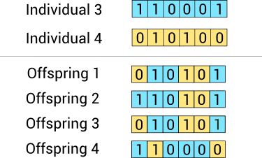
      Crossover Illustration

  • Mutation
    • The crossover operator can generate offsprings that are very similar to the parents. This might cause a new generation with low diversity.
    • The mutation operator solves this problem by changing the value of some features in the offsprings at random.
    • To decide if a feature is mutated, we generate a random number between 0 and 1. If this number is lower than a value called the mutation rate, that variable is flipped.
    • The mutation rate is usually chosen to be 1/m, where m is the number of features. With that value, we mutate one feature of each individual (statistically).

2. Pros & Cons

Pros

• Genetic algorithms can manage data sets with many features.
• They don't need specific knowledge about the problem under study.
• These algorithms can be easily parallelized in computer clusters.

Cons

• Genetic Algorithms might be costly in computational terms since the evaluation of each individual requires the training of a model.
• These algorithms can take a long time to converge since they have a stochastic nature.

3. Application

• If the space to be searched is not so well understood and relatively unstructured (e.g. non-convex, undifferentiable, etc), and if an effective GA representation of that space can be developed, GA is good for usage
• They’re best for problems where there is a clear way to evaluate fitness.
• If the base algorithm's computation is expensive, it is not advisable to use this method
• It is rather rare to use, if you want, checkout this notebook using deap as the package for GA

Some tools to use

1. Scikit learn

• Random Search
• Grid Search

2. HyperOpt

• Random Search
• Tree of Parzen Estimators (TPE)
• Adaptive TPE

3. Optuna

• Most BO algorithms contained
• Pruning feature which automatically stops the unpromising trails in the early stages of training

4. Ray Tune

• ASHA, BOHB
• Distributed asynchronous automatically
• Very Scalable
• Supports Tensorboard and MLflow.
• Supports a variety of frameworks such sklearn, xgboost, Tensorflow, pytorch, etc.

Conclusion

For engineers, it is really matter of choices based on the nature of your code/project. However, for researchers, what optimization strategy you choose could directly affect the theoretical performance of the algorithm. Hence it is worth reading more into the topic of Bayesian Optimization and Sequential decision-making problems. I will also update my posts on BO/Bandit later.