Topic Modeling with Latent Dirichlet Allocation

Overview

Topic modeling: Topic modelling refers to the task of identifying topics that best describes a set of documents. In this blog, we discuss about an popular advanced model that

Definition

• To explain in plain word:

  LDA imagines a fixed set of topics. Each topic represents a set of words. The goal of LDA is to map all the documents to the topics in a way, such that the words in each document are mostly captured by those imaginary topics.

• An important note to take is that LDA aims to explain the document-level idea, meaning it has less focus on the meaning of each word/phrase in the document, but rather the topic the document falls under

• Dirichlet Process:

  • A family of stochastic process to produce a probability distribution
  • Used in Bayesian Inference to describe the prior knowledge about the distribution of random variables

• Dirichlet Distribution:

  • Basically a multivariate generalisation of the Beta distribution: where is a beta distribution
  • Outputs: where
  • Often called “a distribution of distribution”
  • symmetric Dirichlet distribution: a special case in the Dirichlet distribution where all are equal, hence use a single scalar in the model representation
  • Impact of : (a scaling vector for each dimension in )
    • :
      • Sparsity increases
      • The distribution is likely bowl-shaped (most probable vectors are sparse vectors like or
      • In LDA, it means a document is likely to be represented by just a few of the topics
    • • Sparcity decreases
      • We will have a unimodel distribution (most probable vectors are in the center)
      • In LDA, it means a document is likely to contain most of the topics makes documents more similar to each other
    • The conjugate prior of multinomial distribution is a Dirichlet distribution

• LDA\s keywords

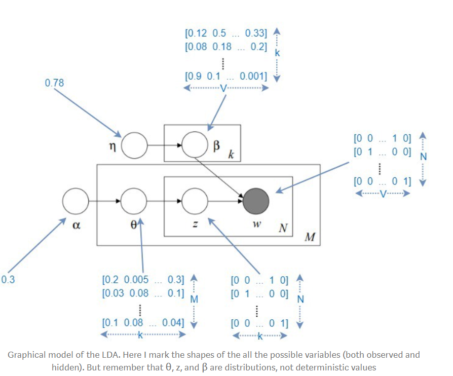
  • k: Number of topics a document belongs to (a fixed number)
  • V : Size of the vocabulary
  • M: Number of documents
  • N: Number of words in each document
  • w: A word in a document. This is represented as a one hot encoded vector of size V
  • W: represents a document (i.e. vector of "w"s) of N words
  • D: Corpus, a collection of M documents
  • z: A topic from a set of k topics. A topic is a distribution words. For example it might be, Animal = (0.3 Cats, 0.4 Dogs, 0 AI, 0.2 Loyal, 0.1 Evil)
  • θ: The topic distribution for each of the document based on a parameter α
  • β: The Dirichlet distribution based on parameter η

LDA's procedure

• This is quite complicated

• LDA's document generation

  

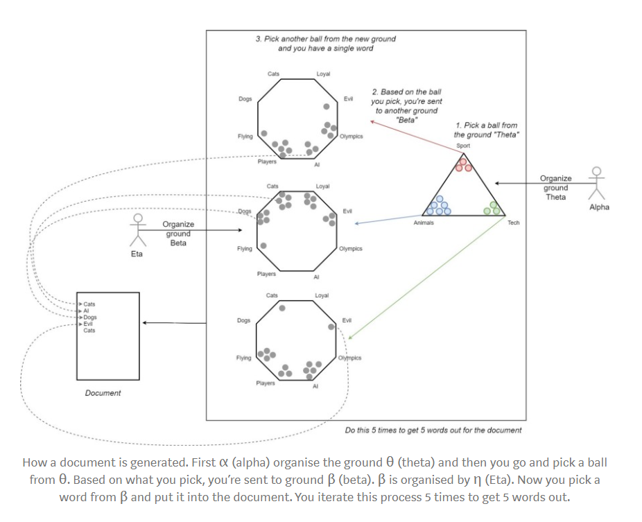
  • α has a topic distribution for each document (θ ground for each document) a (M x K) shape matrix
  • η has a parameter vector for each topic. η will be of shape (k x V)
  • In the above drawing, the constants actually represent matrices, and are formed by replicating the single value in the matrix to every single cell.
  • θ is a random matrix based on dirichlet distribution, where represents the probability of the th document to containing words belonging to the th topic a relatively low
  • β is also a dirichlet distribution as θ, represents the probability of the th topic containing the th word in a vocabulary of size ; The higher the , the more th topic is likely to contain more of the words, and makes the topics more similar to each other
  • Detailed steps:
    1. For each topic, draw a distribution over words
    2. For each document
       1. Draw a vector of topic proportions . E.g: [climate = 0.7, trade = 0.2, housing = 0.1, economy = 0]
       2. For each word slot allocated, draw a topic assignment , then draw a word
    3. We want to infer the join probability given our observations,
       • We infer the hidden variables or latent factors by observing the corpse of documents, i.e. finding

• The learning part

  

  • Idea 1: Gibbs sampling:

    • A point-wise method (Possible but not optimal)

    • Intuition: The setting which generates the original document with the highest proability is the optimal machine

    • The mathematics of collapsed gibbs sampling (cut back version)
      Recall that when we iterate through each word in each document, we unassign its current topic assignment and reassign the word to a new topic. The topic we reassign the word to is based on the probabilities below.

      where

      - number of word assignments to topic in document

      - number of assignments to topic in document

      - smoothing parameter (hyper parameter - make sure probability is never 0)

      - number of words in document

      - don’t count the current word you’re on

      - total number of topics

      - number of assignments, corpus wide, of word to topic

      - number of assignments, corpus wide, of word to topic

      - smoothing parameter (hyper parameter - make sure probability is never 0)

      - sum over all words in vocabulary currently assigned to topic

      size of vocabulary i.e. number of distinct words corpus wide

    • Done with each word in a document (to classify them into a topic)

    • Done in an iterative way (different topics for same words in a document: 1st "happy" may be topic 1, which affects 2nd "happy" to be topic 2 in the same document)

    • Main steps:

      • For each word in a document :
      • The word will be allocated to
      • Note that is the one used in the original and in
      • Iterate until each document & word's topic is upadted
      • Aggregate the results from all documents to update the word distribution for each topic
      • Repeat the previous steps until corpus objective converges

  • Idea 2: variational inference:

    • The key concept of variance inference is approximate posterior with a distribution using some known families of distribution that is easy to model and to analyze.
    • Then, we train the model parameters to minimize the KL-divergence between q and p.
    • KL-divergence: ,also called "relative entropy"
    • Further reduction in complexity for high dimensional distribution is possible

  • Idea 3: Mean-field variational inference

    • breaks up the joint distribution into distributions of individual variables that are tractable and easy to analyze

      

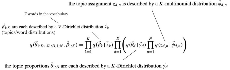
    • It is not easy to optimize KL-divergence directly. So let us introduce the Evidence lower bound (ELBO)

      • by maximizing ELBO, we are minimizing KL-divergence: view explanation here
        • When minimizing ELBO, we don’t need Z. No normalization is needed. In contrast, KL’s calculation needs the calculated entity to be a probability distribution. Therefore, we need to compute the normalization factor Z if it is not equal to one. Calculating Z is hard. This is why we calculate ELBO instead of KL-divergence.

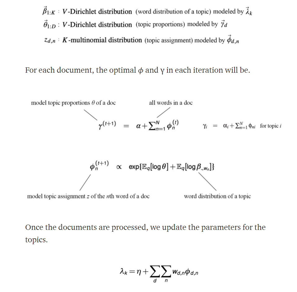
    • There are a lot of math details involving exponential family operations, but the general picutre is captured by the graph below

    

• Evaluation using similarity query

  Ok, now that we have a topic distribution for a new unseen document, let's say we wanted to find the most similar documents in the corpus. We can do this by comparing the topic distribution of the new document to all the topic distributions of the documents in the corpus. We use the Jensen-Shannon distance metric to find the most similar documents.

  What the Jensen-Shannon distance tells us, is which documents are statisically "closer" (and therefore more similar), by comparing the divergence of their distributions. Jensen-Shannon is symmetric, unlike Kullback-Leibler on which the formula is based. This is good, because we want the similarity between documents A and B to be the same as the similarity between B and A.

  The formula is described below.

  For discrete distirbutions and , the Jensen-Shannon divergence, is defined as

  where

  and is the Kullback-Leibler divergence

  The square root of the Jensen-Shannon divergence is the Jensen-Shannon Distance:

  The smaller the Jensen-Shannon Distance, the more similar two distributions are (and in our case, the more similar any 2 documents are)

Pros & Cons

Pros

• An effective tool for topic modeling
• Easy to understand/interpretable
• variational inference is tractable
• θ are document-specific, so the variational parameters of θ could be regarded as the representation of a document , hence the feature set is reduced.
• z are sampled repeatedly within a document — one document can be associated with multiple topics.

Cons

• Must know the number of topics K in advance
• Hard to know when LDA is working - topics are soft-clusters so there is no objective metric to say "this is the best choice" of hyperparameters
• LDA does not work well with very short documents, like twitter feeds
• Dirichlet topic distribution cannot capture correlations among topics
• Stopwords and rare words should be excluded, so that the model doesnt overcompensate for very frequent words and very rare words, both of which do not contribute to general topics.

Real-word application

• Text classification

• Book recommender

• Article clustering/image clustering

• understanding the different varieties topics in a corpus (obviously)

• getting a better insight into the type of documents in a corpus (whether they are about news, wikipedia articles, business documents)

• quantifying the most used / most important words in a corpus

• document similarity and recommendation.

Long Code example

# import dependencies
%matplotlib inline
import pandas as pd
import numpy as np
import nltk
from nltk.corpus import stopwords
import gensim
from gensim.models import LdaModel
from gensim import models, corpora, similarities
import re
from nltk.stem.porter import PorterStemmer
import time
from nltk import FreqDist
from scipy.stats import entropy
import matplotlib.pyplot as plt
import seaborn as sns

# Read in data; only keep essential columns and English language articles
df = pd.read_csv('lda_fake.csv', usecols = ['uuid','author','title','text','language','site_url','country'])
df = df[df.language == 'english']
df = df[df['text'].map(type) == str]
df['title'].fillna(value="", inplace=True)
df.dropna(axis=0, inplace=True, subset=['text'])
# shuffle the data
df = df.sample(frac=1.0)
df.reset_index(drop=True,inplace=True)

# Define some functions to clean and tokenize the data
def initial_clean(text):
    """
    Function to clean text of websites, email addresess and any punctuation
    We also lower case the text
    """
    text = re.sub("((\S+)?(http(s)?)(\S+))|((\S+)?(www)(\S+))|((\S+)?(\@)(\S+)?)", " ", text)
    text = re.sub("[^a-zA-Z ]", "", text)
    text = text.lower() # lower case the text
    text = nltk.word_tokenize(text)
    return text

stop_words = stopwords.words('english')
def remove_stop_words(text):
    """
    Function that removes all stopwords from text
    """
    return [word for word in text if word not in stop_words]

stemmer = PorterStemmer()
def stem_words(text):
    """
    Function to stem words, so plural and singular are treated the same
    """
    try:
        text = [stemmer.stem(word) for word in text]
        text = [word for word in text if len(word) > 1] # make sure we have no 1 letter words
    except IndexError: # the word "oed" broke this, so needed try except
        pass
    return text

def apply_all(text):
    """
    This function applies all the functions above into one
    """
    return stem_words(remove_stop_words(initial_clean(text)))

# clean text and title and create new column "tokenized"
t1 = time.time()
df['tokenized'] = df['text'].apply(apply_all) + df['title'].apply(apply_all)
t2 = time.time()
print("Time to clean and tokenize", len(df), "articles:", (t2-t1)/60, "min")

# We'll use nltk to get a word frequency (by count) here and only keep the top most used words to train the LDA model on

# first get a list of all words
all_words = [word for item in list(df['tokenized']) for word in item]
# use nltk fdist to get a frequency distribution of all words
fdist = FreqDist(all_words)
len(fdist) # number of unique words

# choose k and visually inspect the bottom 10 words of the top k
k = 50000
top_k_words = fdist.most_common(k)
top_k_words[-10:]

# choose k and visually inspect the bottom 10 words of the top k
k = 15000
top_k_words = fdist.most_common(k)
top_k_words[-10:]

# k = 50,000 is too high, as the bottom words aren't even real words and are very rarely used (once in entire corpus)

# k = 15,000 is much more reasonable as these have been used at least 13 times in the corpus

# define a function only to keep words in the top k words
top_k_words,_ = zip(*fdist.most_common(k))
top_k_words = set(top_k_words)
def keep_top_k_words(text):
    return [word for word in text if word in top_k_words]
	
df['tokenized'] = df['tokenized'].apply(keep_top_k_words)

# document length
df['doc_len'] = df['tokenized'].apply(lambda x: len(x))
doc_lengths = list(df['doc_len'])
df.drop(labels='doc_len', axis=1, inplace=True)

print("length of list:",len(doc_lengths),
      "\naverage document length", np.average(doc_lengths),
      "\nminimum document length", min(doc_lengths),
      "\nmaximum document length", max(doc_lengths))
	  
# plot a histogram of document length
num_bins = 1000
fig, ax = plt.subplots(figsize=(12,6));
# the histogram of the data
n, bins, patches = ax.hist(doc_lengths, num_bins)
ax.set_xlabel('Document Length (tokens)', fontsize=15)
ax.set_ylabel('Normed Frequency', fontsize=15)
ax.grid()
ax.set_xticks(np.logspace(start=np.log10(50),stop=np.log10(2000),num=8, base=10.0))
plt.xlim(0,2000)
ax.plot([np.average(doc_lengths) for i in np.linspace(0.0,0.0035,100)], np.linspace(0.0,0.0035,100), '-',
        label='average doc length')
ax.legend()
ax.grid()
fig.tight_layout()
plt.show()

### Drop short articles

LDA does not work very well on short documents, which we will explain later, so we will drop some of the shorter articles here before training the model.

From the histogram above, droping all articles less than 40 tokens seems appropriate.

# only keep articles with more than 30 tokens, otherwise too short
df = df[df['tokenized'].map(len) >= 40]
# make sure all tokenized items are lists
df = df[df['tokenized'].map(type) == list]
df.reset_index(drop=True,inplace=True)
print("After cleaning and excluding short aticles, the dataframe now has:", len(df), "articles")

# create a mask of binary values
msk = np.random.rand(len(df)) < 0.999

train_df = df[msk]
train_df.reset_index(drop=True,inplace=True)

test_df = df[~msk]
test_df.reset_index(drop=True,inplace=True)

def train_lda(data):
    """
    This function trains the lda model
    We setup parameters like number of topics, the chunksize to use in Hoffman method
    We also do 2 passes of the data since this is a small dataset, so we want the distributions to stabilize
    """
    num_topics = 100
    chunksize = 300
    dictionary = corpora.Dictionary(data['tokenized'])
    corpus = [dictionary.doc2bow(doc) for doc in data['tokenized']]
    t1 = time.time()
    # low alpha means each document is only represented by a small number of topics, and vice versa
    # low eta means each topic is only represented by a small number of words, and vice versa
    lda = LdaModel(corpus=corpus, num_topics=num_topics, id2word=dictionary,
                   alpha=1e-2, eta=0.5e-2, chunksize=chunksize, minimum_probability=0.0, passes=2)
    t2 = time.time()
    print("Time to train LDA model on ", len(df), "articles: ", (t2-t1)/60, "min")
    return dictionary,corpus,lda
	
dictionary,corpus,lda = train_lda(train_df)

# show_topics method shows the the top num_words contributing to num_topics number of random topics
lda.show_topics(num_topics=10, num_words=20)

# select and article at random from train_df
random_article_index = np.random.randint(len(train_df))
bow = dictionary.doc2bow(train_df.iloc[random_article_index,7])

# get the topic contributions for the document chosen at random above
doc_distribution = np.array([tup[1] for tup in lda.get_document_topics(bow=bow)])

# bar plot of topic distribution for this document
fig, ax = plt.subplots(figsize=(12,6));
# the histogram of the data
patches = ax.bar(np.arange(len(doc_distribution)), doc_distribution)
ax.set_xlabel('Topic ID', fontsize=15)
ax.set_ylabel('Topic Contribution', fontsize=15)
ax.set_title("Topic Distribution for Article " + str(random_article_index), fontsize=20)
ax.set_xticks(np.linspace(10,100,10))
fig.tight_layout()
plt.show()

# select and article at random from test_df
random_article_index = np.random.randint(len(test_df))
print(random_article_index)
new_bow = dictionary.doc2bow(test_df.iloc[random_article_index,7])
print(test_df.iloc[random_article_index,3])

new_doc_distribution = np.array([tup[1] for tup in lda.get_document_topics(bow=new_bow)])
# bar plot of topic distribution for this document
fig, ax = plt.subplots(figsize=(12,6));
# the histogram of the data
patches = ax.bar(np.arange(len(new_doc_distribution)), new_doc_distribution)
ax.set_xlabel('Topic ID', fontsize=15)
ax.set_ylabel('Topic Contribution', fontsize=15)
ax.set_title("Topic Distribution for an Unseen Article", fontsize=20)
ax.set_xticks(np.linspace(10,100,10))
fig.tight_layout()
plt.show()

def jensen_shannon(query, matrix):
    """
    This function implements a Jensen-Shannon similarity
    between the input query (an LDA topic distribution for a document)
    and the entire corpus of topic distributions.
    It returns an array of length M where M is the number of documents in the corpus
    """
    # lets keep with the p,q notation above
    p = query[None,:].T # take transpose
    q = matrix.T # transpose matrix
    m = 0.5*(p + q)
    return np.sqrt(0.5*(entropy(p,m) + entropy(q,m)))
	
def get_most_similar_documents(query,matrix,k=10):
    """
    This function implements the Jensen-Shannon distance above
    and retruns the top k indices of the smallest jensen shannon distances
    """
    sims = jensen_shannon(query,matrix) # list of jensen shannon distances
    return sims.argsort()[:k] # the top k positional index of the smallest Jensen Shannon distances
	
# this is surprisingly fast
most_sim_ids = get_most_similar_documents(new_doc_distribution,doc_topic_dist)

most_similar_df = train_df[train_df.index.isin(most_sim_ids)]
most_similar_df['title']