MLOps Post-Training Considerations

Introduction

Training a model is only the middle of an ML system. After training, the team still needs to preserve the experiment, store the model artifact, deploy it behind a reliable interface, and monitor whether it continues to behave well in production.

This post is a practical map of the post-training lifecycle:

• Experiment tracking: save metrics, parameters, artifacts, logs, and environment details.
• Model registry: version trained models and define which artifacts are candidates for production.
• Model serving: expose the model through online, batch, streaming, or serverless workflows.
• Monitoring: track model behavior, system health, resource usage, and drift.

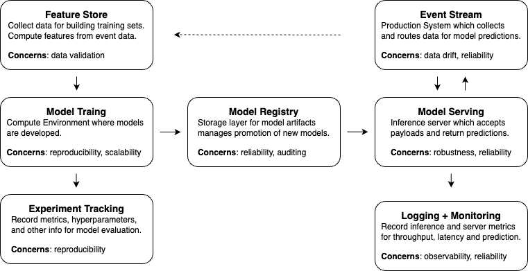
The details can become deep quickly, so this post focuses on the main design decisions rather than every tool-specific setup step.

Experiment Tracking

Experiment tracking makes model development reproducible and comparable. Without it, the team can lose track of which dataset, code version, hyperparameters, metric implementation, and environment produced a result.

Good tracking should capture:

• Parameters: model settings, training settings, feature settings, prompt versions, or retrieval settings.
• Metrics: training metrics, validation metrics, slice metrics, latency, and cost.
• Artifacts: trained weights, plots, reports, evaluation outputs, sample predictions, and logs.
• Code and data versions: git commit, data snapshot, feature schema, and label source.
• Environment: package versions, Docker image, hardware, and runtime configuration.

Common tools include MLflow, Weights & Biases, Neptune, TensorBoard, and cloud-native experiment trackers.

MLflow Example

MLflow is a common default because it covers experiment tracking and model registry workflows.

from datetime import datetime

import mlflow


experiment_name = "credit-risk"
run_name = datetime.now().strftime("%Y%m%d-%H%M")

mlflow.set_tracking_uri("http://localhost:5000")
mlflow.set_experiment(experiment_name)

with mlflow.start_run(run_name=run_name):
    mlflow.log_param("model_type", "random_forest")
    mlflow.log_param("n_estimators", 200)

    # Train and evaluate the model.
    model = train_model()
    metrics = evaluate_model(model)

    mlflow.log_metric("validation_auc", metrics["auc"])
    mlflow.log_artifact("reports/confusion_matrix.png")

The exact API depends on the model framework, but the design principle is stable: a run should tell you what happened, what it produced, and whether it is worth comparing to another run.

Tracking Configuration

Configuration should be stored as a first-class artifact. A plain YAML file is often enough:

project: home-credit-default-risk

data:
  n_cv_splits: 5
  validation_size: 0.2
  stratified_cv: true

model:
  type: random_forest
  n_estimators: 2000
  max_depth: 40
  min_samples_split: 50
  class_weight: balanced

post_processing:
  aggregation_method: rank_mean

Load it safely:

import yaml


with open(config_path, "r", encoding="utf-8") as file:
    config = yaml.safe_load(file)

print(config["data"]["n_cv_splits"])

For larger projects, Hydra can help compose environment-specific configs:

import hydra
from omegaconf import DictConfig, OmegaConf


@hydra.main(version_base=None, config_path="conf", config_name="config")
def train(cfg: DictConfig) -> None:
    print(OmegaConf.to_yaml(cfg))
    print(cfg.model.n_estimators)


if __name__ == "__main__":
    train()

Tracking Data and Environment

Data is harder to version than code because it may live in object storage, databases, feature stores, or vendor systems. Use a data registry or versioning layer when the dataset matters for reproducibility. DVC, lakehouse tables, feature stores, and cloud experiment platforms can all play this role.

The runtime environment should also be recoverable. Docker is usually the most reliable option:

FROM python:3.11-slim

WORKDIR /app
COPY pyproject.toml README.md ./
COPY src ./src

RUN python -m pip install --upgrade pip \
    && python -m pip install -e .

CMD ["python", "-m", "your_project.train"]

Conda or uv can also work. The important part is that the environment is described explicitly and stored with the experiment or model artifact.

Model Registry

A model registry stores trained model artifacts and their metadata. It answers questions like:

• Which model versions exist?
• Which version is approved for staging or production?
• Which code, data, and config produced this artifact?
• Which evaluation results justify promotion?
• How can we roll back?

Some teams keep registry functionality inside MLflow or a cloud ML platform. Others use object storage plus metadata tables. The implementation matters less than the contract: a production model should never be a mystery file on someone’s machine.

Development vs Production Registries

Development registries are optimized for iteration:

• Many model versions
• More open write access
• Exploratory runs and failed experiments
• Debugging artifacts and richer metadata

Production registries are optimized for reliability:

• Fewer approved model versions
• Stronger access control
• Promotion gates and audit history
• Champion and challenger models
• Rollback-ready artifacts

The two environments can use the same tool, but they should not have the same permissions or promotion rules.

Save, Package, Register

It helps to separate three actions:

• Save: write model state locally or to object storage.
• Package: bundle the model with code, dependencies, schemas, and runtime requirements.
• Register: store the artifact and metadata in a system that the team can search, promote, deploy, and audit.

For PyTorch, saving model state may look like this:

import torch


checkpoint = {
    "model_state": model.state_dict(),
    "optimizer_state": optimizer.state_dict(),
    "config": config,
}

torch.save(checkpoint, "model.pt")

For serving across runtimes, packaging might involve ONNX, TorchScript, a Python wheel, or a Docker image. For registry, MLflow can log and register framework-specific models:

import mlflow


with mlflow.start_run():
    mlflow.log_params(config)
    mlflow.sklearn.log_model(
        sk_model=model,
        artifact_path="model",
        registered_model_name="credit-risk-model",
    )

Model Serving

Model serving turns a trained model into a usable product capability. The simplest version loads a model, transforms input features, runs inference, and returns predictions. Production serving adds schemas, latency budgets, scaling, error handling, logging, and rollback.

Common serving modes:

• Online: synchronous request-response inference for user-facing features.
• Batch: scheduled inference over many records.
• Streaming: inference or feature processing over event streams.
• Offline: precomputed embeddings, rankings, recommendations, or scores.
• Serverless: managed endpoints where the cloud provider handles much of the scaling.

API Architecture

Three common interface styles are REST, gRPC, and WebSocket.

REST is simple, widely supported, and easy to debug. It is often the best default for prediction endpoints that do not require streaming.

gRPC is efficient and strongly typed. It is useful when low latency, internal service communication, or streaming matters.

WebSocket supports long-lived bidirectional communication. It is useful for real-time updates, but connection management is more complex.

Pick the interface based on the product path, not based on novelty. A recommendation batch job, an LLM streaming chat endpoint, and a fraud-scoring service may all need different serving patterns.

Online and Offline Together

Many ML systems mix online and offline inference. A recommender system might precompute candidate embeddings offline, then do final ranking online. A search system might refresh document embeddings in batch, then use them for real-time retrieval.

This split can reduce latency and cost, but it introduces a contract: the online service must know which offline artifacts, feature versions, and embedding versions it is using.

ETL-Based Deployment

ETL-style deployment is useful when predictions do not need to happen in real time. The job extracts records, transforms features, runs inference, and loads results into a destination table or storage system.

This fits:

• Daily risk scores
• Batch recommendations
• Scheduled document enrichment
• Offline feature generation
• Backfills and reprocessing jobs

Tools such as Airflow, Apache Beam, Spark, and cloud batch systems are often better for this than a web server.

Event-Driven Serving

In a larger distributed system, model inference may be triggered by messages rather than HTTP requests. Kafka, RabbitMQ, Celery, or cloud queues can decouple producers from inference workers.

This is useful when inference can be asynchronous, when workloads spike, or when multiple downstream consumers need the same prediction event.

Model Monitoring

Monitoring ML systems has three layers.

Model metrics

• Prediction distributions
• Feature distributions
• Evaluation metrics when ground truth becomes available
• Segment-level performance
• Drift signals

System metrics

• Request throughput
• Error rate
• Request latency
• Request body size
• Response body size
• Timeout and retry counts

Resource metrics

• CPU utilization
• Memory utilization
• GPU utilization
• Network transfer
• Disk I/O

Software monitoring tells you whether the service is healthy. Model monitoring tells you whether the predictions are still useful.

Prometheus and Grafana Pattern

Jeremy Jordan’s monitoring example uses a practical open-source stack: expose a model service through FastAPI, instrument it with metrics, collect those metrics with Prometheus, visualize them with Grafana, and simulate traffic with Locust.

The general flow is:

1. Create a containerized model service with prediction and health endpoints.
2. Expose metrics through a /metrics endpoint.
3. Configure Prometheus to scrape the metrics endpoint.
4. Build Grafana dashboards for model, system, and resource metrics.
5. Use load testing to generate traffic before relying on production dashboards.

For Kubernetes, Prometheus can discover scrape targets through service discovery or explicit service monitors:

endpoints:
  - path: /metrics
    port: app
    interval: 15s

Drift Detection

Drift detection can be handled in several ways:

• Run a drift-detection service beside the model.
• Log statistical profiles of production features.
• Store sampled feature payloads for later analysis.
• Compare online feature distributions against training or validation distributions.
• Compute delayed evaluation metrics when labels arrive.

Be careful with what you store. Full payload logging can be useful for debugging, but it may create privacy, cost, and compliance problems.

Monitoring Practices

For Prometheus:

• Avoid high-cardinality labels.
• Use unit suffixes in metric names, such as _seconds or _bytes.
• Use base units when possible.
• Prefer standard exporters when they exist.

For Grafana:

• Keep dashboards discoverable and consistent.
• Use template variables instead of duplicating dashboards.
• Put important context near the chart.
• Store dashboard definitions in source control.
• Avoid dashboards nobody owns.

Summary

Post-training work is where a model becomes a system. The important questions are practical:

• Can we reproduce the experiment?
• Can we find and promote the right model artifact?
• Can the serving path meet product requirements?
• Can we detect when the service or model behavior gets worse?
• Can we roll back safely?

The more serious the model’s product role becomes, the more these post-training practices matter.

References

• Jeremy Jordan: A simple solution for monitoring ML systems
• MLflow tracking documentation
• AWS: Track ML experiments end to end with DVC and SageMaker Experiments
• Prometheus exporters and integrations