Clustering: Affinity Propagation

Affinity Propagation Introduction

• Developed recently (2007), a centroid based clustering algorithm similar to k Means or K medoids

• Affinity propagation finds "exemplars" i.e. members of the input set that are representative of clusters.

• It uses a graph based approach to let points 'vote' on their preferred 'exemplar'. The end result is a set of cluster 'exemplars' from which we derive clusters by essentially doing what K-Means does and assigning each point to the cluster of it's nearest exemplar.

• We need to calculate the following matrices:
  Here we must specify to notation: = row, = column

  1. Similarity matrix
  2. Responsibility matrix
  3. Availability matrix
  4. Criterion matrix

• Similarity matrix

  • Rationale: information about the similarity between any instances, for an element i we look for another element j for which is the highest (least negative). Hence the diagonal values are all set to the most negative to exclude the case where i find i itself
  • Barring those on the diagonal, every cell in the similarity matrix is calculated by the negative sum of the squares differences between participants.
  • Note that the diagonal values will not be just 0: It is

• Responsibility matrix

  • Rationale: quantifies how well-suited element k is, to be an exemplar for element i , taking into account the nearest contender k’ to be an exemplar for i.

  • We initialize R matrix with zeros.

  • Then calculate every cell in the responsibility matrix using the following formula:

    • Interpretation: R_{i,k} can be thought of as relative similarity between i and k. It quantifies how similar is i to k, compared to some k’, taking into account the availability of k’. The responsibility of k towards i will decrease as the availability of some other k’ to i increases.

• Availability matrix

  • Rationale: It quantifies how appropriate is it for i to choose k as its exemplar, taking into account the support from other elements that k should an exemplar.
  • The Availability formula for different instances is
  • The Self-Availability is
  • Interpretation of the formulas
    • Availability is self-responsibility of k plus the positive responsibilities of k towards elements other than i.
    • We include only positive responsibilities as an exemplar should be positively responsible/explain at least for some data points well, regardless of how poorly it explains other data points.
    • If self-responsibility is negative, it means that k is more suitable to belong to another exemplar, rather than being an exemplar. The maximum value of is 0.
    • reflects accumulated evidence that point k is suitable to be an exemplar, based on the positive responsibilities of k towards other elements.

• and matrices are iteratively updated. This procedure may be terminated after a fixed number of iterations, after changes in the values obtained fall below a threshold, or after the values stay constant for some number of iterations.

• Criterion Matrix

  • Criterion matrix is calculated after the updating is terminated.
  • Criterion matrix is the sum of and :
  • An element i will be assigned to an exemplar k which is not only highly responsible but also highly available to i.
  • The highest criterion value of each row is designated as the exemplar. Rows that share the same exemplar are in the same cluster.

• Sample run

  

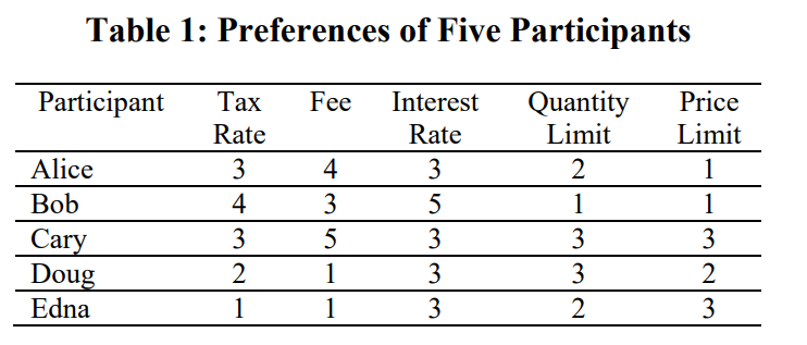
  Data

  

  Similarity Matrix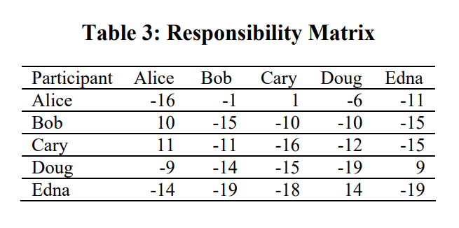

  

  Responsibility Matrix (First round)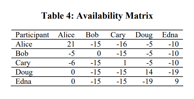

  

  Availability Matrix (First round)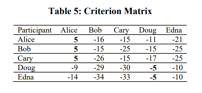

  

  Criterion Matrix

2. Pros & Cons

Pros

• Does not need to specify the cluster number
• Allows for non-metric dissimilarities (i.e. we can have dissimilarities that don't obey the triangle inequality, or aren't symmetric)
• Providebetter stability over runs

Cons

• Similar issue as K-means: susceptible to outliers
• Affinity Propagation tends to be very slow. In practice running it on large datasets is essentially impossible without a carefully crafted and optimized implementation

3. Code Implementation

from sklearn.cluster import AffinityPropagation
from sklearn import metrics
from sklearn.datasets import make_blobs

# #############################################################################
# Generate sample data
centers = [[1, 1], [-1, -1], [1, -1]]
X, labels_true = make_blobs(n_samples=300, centers=centers, cluster_std=0.5,
                            random_state=0)

# #############################################################################
# Compute Affinity Propagation
af = AffinityPropagation(preference=-50).fit(X)
cluster_centers_indices = af.cluster_centers_indices_
labels = af.labels_

n_clusters_ = len(cluster_centers_indices)

print('Estimated number of clusters: %d' % n_clusters_)
print("Homogeneity: %0.3f" % metrics.homogeneity_score(labels_true, labels))
print("Completeness: %0.3f" % metrics.completeness_score(labels_true, labels))
print("V-measure: %0.3f" % metrics.v_measure_score(labels_true, labels))
print("Adjusted Rand Index: %0.3f"
      % metrics.adjusted_rand_score(labels_true, labels))
print("Adjusted Mutual Information: %0.3f"
      % metrics.adjusted_mutual_info_score(labels_true, labels))
print("Silhouette Coefficient: %0.3f"
      % metrics.silhouette_score(X, labels, metric='sqeuclidean'))

# #############################################################################
# Plot result
import matplotlib.pyplot as plt
from itertools import cycle

plt.close('all')
plt.figure(1)
plt.clf()

colors = cycle('bgrcmykbgrcmykbgrcmykbgrcmyk')
for k, col in zip(range(n_clusters_), colors):
    class_members = labels == k
    cluster_center = X[cluster_centers_indices[k]]
    plt.plot(X[class_members, 0], X[class_members, 1], col + '.')
    plt.plot(cluster_center[0], cluster_center[1], 'o', markerfacecolor=col,
             markeredgecolor='k', markersize=14)
    for x in X[class_members]:
        plt.plot([cluster_center[0], x[0]], [cluster_center[1], x[1]], col)

plt.title('Estimated number of clusters: %d' % n_clusters_)
plt.show()