Agglomerative : This is a "bottom-up" approach: each observation starts in its own cluster, and pairs of clusters are merged as one moves up the hierarchy.
Divisive : This is a "top-down" approach: all observations start in one cluster, and splits are performed recursively as one moves down the hierarchy.
Agglomerative Clustering
Initially each data point is considered as an individual cluster. At each iteration, the most similar clusters merge with other clusters until 1/ K clusters are formed.
No need to specify number of clusters, performance
In sklearn, if we specify the number of clusters, performance can be improved
Procedure
Compute the proximity matrix
Let each data point be a cluster
Repeat: Merge two closest clusters and update the proximity matrix until 1/ K cluster remains
Divisive Clustering
Opposite of agglomerative clustering. We start with one giant cluster including all data points. Then data points are separated into different clusters.
Similarity score:
Basically the proximity between two clusters
Distance calculation
Euclidean Distance
Squared Euclidean Distance
Manhattan Distance
Maximum Distance:
Mahalanobis Distance: where is Covariance matrix
For text or other non-numeric data, metrics such as the Hamming distance or Levenshtein distance are often used.
For details, see Distance metrics & Evaluation method[Unsupervised Learning/0. Distance metrics and Evaluation Methods/Distance_Metrics_Evaluation_Methods.ipynb]
Distance references
Complete-linkage: The maximum distance between elements of each cluster
Single-linkage: The minimum distance between elements of each cluster
Average linkage: The mean distance between elements of each cluster
Ward’s linkage: Minimizes the variance of the clusters being merged. Least increase in total variance around cluster centroids is aimed.
2. Pros & Cons
Pros
Do not have to specify the number of clusters beforehand
It is easy to implement and interpretable with the help of dendrograms
Always generates the same clusters (Stability)
Cons
Exponential runtime for larger datasets
3. Application
Text grouping: However, it is a highly complex task due the high-dimensionality of data.
import numpy as np import pandas as pd import matplotlib.pyplot as plt
from sklearn.cluster import AgglomerativeClustering from sklearn.preprocessing import StandardScaler, normalize from sklearn.decomposition import PCA from sklearn.metrics import silhouette_score import scipy.cluster.hierarchy as shc
# Standardize data scaler = StandardScaler() scaled_df = scaler.fit_transform(raw_df) # Normalizing the Data normalized_df = normalize(scaled_df) # Converting the numpy array into a pandas DataFrame normalized_df = pd.DataFrame(normalized_df) # Reducing the dimensions of the data pca = PCA(n_components = 2) X_principal = pca.fit_transform(normalized_df) X_principal = pd.DataFrame(X_principal) X_principal.columns = ['P1', 'P2']
# Visualizing the clustering plt.scatter(X_principal['P1'], X_principal['P2'], c = AgglomerativeClustering(n_clusters = 3).fit_predict(X_principal), cmap =plt.cm.winter) plt.show()
BIRCH Clustering
1. Definition
Balanced Iterative Reducing and Clustering using Hierarchies (BIRCH)
Rationale: Existing data clustering methods do not adequately address the problem of processing large datasets with a limited amount of resources (i.e. memory and cpu cycles). In consequence, as the dataset size increases, they scale poorly in terms of running time, and result quality.
Main logic of BIRCH:
Deals with large datasets by first generating a more compact summary that retains as much distribution information as possible, and then clustering the data summary instead of the original dataset
Metric attributes
Definition: values can be represented by explicit Euclidean coordinates (no categorical variables).
BIRCH can only deal with metric attributes
Clustering Features
BIRCH summarize the information contained in dense regions as Clustering Feature (CF);
where = # of data points in a cluster, = linear sum of data; = square sum of data;
CF additivity theorem: ;
CF Tree
Clustering Feature tree structure is similar to the balanced B+ tree
A very compact representation of the dataset because each entry in a leaf node is not a single data point but a subcluster.
Each non-leaf node contains at most entries.
Each leaf node contains at most entries, and each entry is a CF
Threshold for leaf entry: all sample points in this CF must be in the radius In a hyper-sphere less than T.
Insertion Algo: (Insert a new CF/Point entry in to the tree)
Starting from the root, recursively traverse down the tree by choosing the node that has shortest Euclidean distance to the inserted entry;
Upon reaching a leaf node, find the shorest distance CF and see if it can include the new CF/Point into the cluster without radius threshold violation; If can: do not create a new leaf, but update all the CF triplets on the path, the insertion ends; If cannot: go to 3;
If the number of CF nodes of the current leaf node is less than the threshold , create a new CF node, put in a new sample and the new CF node into this leaf node, update all CF triplets on the path, and insertion Ends. Otherwise, go to 4
If the leaf node has > L entires after addition, then split the leaf node by choosing the 2 entries that are farthest apart and redistribute CF based on distance to each of the 2 entries;
Modify the path to leaf: Since the leaf node is updated, we need to update the entire path from root to leaf; In the event of split, we need to insert a nonleaf entry into the parent node, and if parent node has > nodes, then we need to split again; do so until it reaches the root
Complete procedure
Phase 1: The algorithm starts with an initial threshold value (ideally start from low), scans the data, and inserts points into the tree. If it runs out of memory before it finishes scanning the data, it increases the threshold value, and rebuilds a new, smaller CF-tree, by re-inserting the leaf entries of the old CF-tree into the new CF-tree. After all the old leaf entries have been re-inserted, the scanning of the data and insertion into the new CF-tree is resumed from the point at which it was interrupted.
(Optional) Filter the CF Tree created in the first step to remove some abnormal CF nodes.
(Optional) Use other clustering algorithms such as K-Means to cluster all CF tuples to get a better CF Tree.
Phase 2: Given that certain clustering algorithms perform best when the number of objects is within a certain range, we can group crowded subclusters into larger ones resulting in an overall smaller CF-tree.
Phase 3: Almost any clustering algorithm can be adapted to categorize Clustering Features instead of data points. For instance, we could use KMEANS to categorize our data, all the while deriving the benefits from BIRCH
Additional passes over the data to correct inaccuracies caused by the fact that the clustering algorithm is applied to a coarse summary of the data.
The complexity of the algorithm is
2. Pros & Cons
Pros
Save memory, all samples are on disk, CF Tree only stores CF nodes and corresponding pointers.
The clustering speed is fast, and it only takes one scan of the training set to build the CF Tree, and the addition, deletion, and modification of the CF Tree are very fast.
Noise points can be identified, and preliminary classification pre-processing can be performed on the data set.
Cons
There is need to specify number of clusters;
The clustering result may be different from the real category distribution.
Does not perform well on non-convex dataset distribution
Apart from number of clusters we have to specify two more parameters;
Birch doesn’t perform well on high dimensional data (if there are >20 features, you’d better use something else).
3. Applications
If the dimension of the data features is very large, such as greater than 20, BIRCH is not suitable. At this time, Mini Batch K-Means performs better.
4. Code implementation
1
2
3
4
5
6
7
8
9
10
11
12
13
14
15
16
import numpy as np from matplotlib import pyplot as plt import seaborn as sns sns.set() from sklearn.datasets import make_blobs from sklearn.cluster import Birch
In spectral clustering, data points are treated as nodes of a graph. Thus, spectral clustering is a graph partitioning problem.
The nodes are mapped to a low-dimensional space that can be easily segregated to form clusters.
No assumption is made about the shape/form of the clusters. The goal of spectral clustering is to cluster data that is connected but not necessarily compact or clustered within convex boundaries.
In general, spectral clustering is a generalized version of k-means: it does not assume a circular shape, but apply different affinity functions in its similarity matrix
Procedures
Project data into matrix
Define an Affinity matrix A , using a Gaussian Kernel K or an Adjacency matrix
Construct the Graph Laplacian from A (i.e. decide on a normalization)
Solve the Eigenvalue problem
Select k eigenvectors corresponding to the k lowest (or highest) eigenvalues to define a k-dimensional subspace
Form clusters in this subspace using k-means
Similarity Graph We first create an undirected graph G = (V, E) with vertex set V = {v1, v2, …, vn} = 1, 2, …, n observations in the data.
-neighbourhood Graph:
: Each point is connected to all the points which lie in it’s -radius.
If all the distances between any two points are similar in scale then typically the weights of the edges (i.e. the distance between the two points) are not stored since they do not provide any additional information.
Hence, the graph built is an undirected and unweighted graph.
K-Nearest Neighbours:
: For two vertices and , an edge is directed from to only if is among the k-nearest neighbours of u.
The graph is a weighted and directed graph because it is not always the case that for each u having v as one of the k-nearest neighbours, it will be the same case for v having u among its k-nearest neighbours. To make this graph undirected, one of the following approaches are followed:
Direct an edge from u to v and from v to u if either v is among the k-nearest neighbours of u OR u is among the k-nearest neighbours of v.
Direct an edge from u to v and from v to u if v is among the k-nearest neighbours of u AND u is among the k-nearest neighbours of v.
Fully-Connected Graph:
Each point is connected with an undirected edge-weighted by the distance between the two points to every other point.
Since this approach is used to model the local neighbourhood relationships thus typically the Gaussian similarity metric is used to calculate the distance:
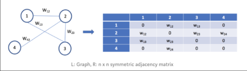
Thus, when we create an adjacency matrix for any of these graphs, when the points are close and if the points are far apart. Consider the following graph with nodes 1 to 4, weights (or similarity) wij and its adjacency matrix:
Adjacency Matrix
Adjacency Matrix
Affinity metric determines how close, or similar, two points our in our space. We will use a Gaussian Kernel and not the standard Euclidean metric.
Given 2 data points (projected in ), we define an Affinity that is positive, symmetric, and depends on the Euclidian distance between the data points
We might provide a hard cut off threshold , so that if
when the points are close in , and if the points , are far apart.
Close data points are in the same cluster. Data points in different clusters are far away. But data points in the same cluster may also be far away–even farther away than points in different clusters. Our goal then is to transform the space so that when 2 points , are close, they are always in same cluster, and when they are far apart, they are in different clusters. Generally we use the Gaussian Kernel K directly, or we form the Graph Laplacian .
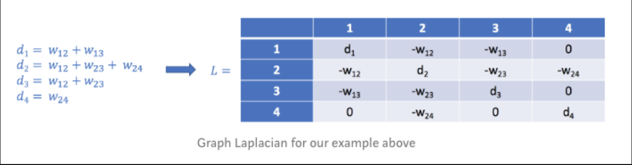
Degree Matrix The degree matrix of a graph is the matrix defined by
where of a vertex is the number of edges that terminate at
Graph Laplacian
The whole purpose of computing the Graph Laplacian was to find eigenvalues and eigenvectors for it, in order to embed the data points into a low-dimensional space.
Just another matrix representation of a graph. It can be computed as:
Simple Laplacian where is the Adjacency matrix and is the Degree Matrix
Normalized Laplacian
Generalized Laplacian
Relaxed Laplacian
Ng, Jordan, & Weiss Laplacian , where
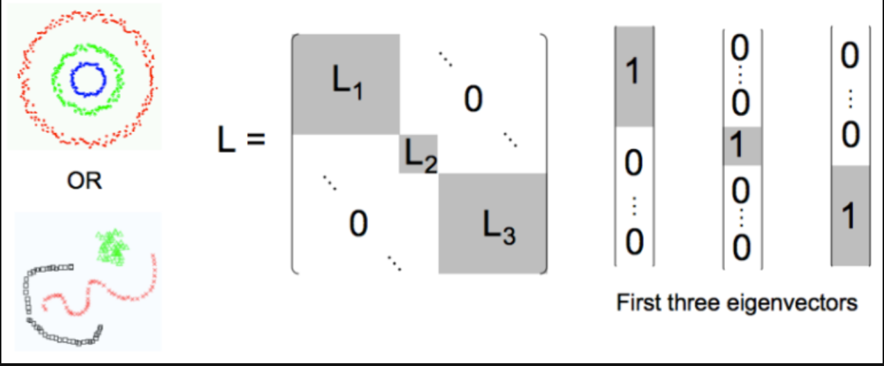
The Cluster Eigenspace Problem
To identify good clusters, Laplacian should be approximately a block-diagonal, with each block defining a cluster. If we have 3 major clusters (C1, C2, C3), we would expect
- We also expect that the 3 lowest eigenvalues & eigenvectors of each correspond to a different cluster.
- For K clusters, compute the first K eigen vectors. . Stack the vectors vertically to form the matrix with eigen vecttors as columns. Represent every node as the corresponding row of this new matrix, these rows form the feature vector of the nodes. Use Kmeans to cluster these points into k clusters
2. Pros & Cons
Pros
Clusters not assumed to be any certain shape/distribution, in contrast to e.g. k-means. This means the spectral clustering algorithm can perform well with a wide variety of shapes of data.
Works quite well when relations are approximately transitive (like similarity)
Do not necessarily need the actual data set, just similarity/distance matrix, or even just Laplacian
Because of this, we can cluster one dimensional data as a result of this; other algos that can do this are k-medoids and heirarchical clustering.
Cons
Need to choose the number of clusters k, although there is a heuristic to help choose
Can be costly to compute, although there are algorithms and frameworks to help
import pandas as pd import matplotlib.pyplot as plt from sklearn.cluster import SpectralClustering from sklearn.preprocessing import StandardScaler, normalize from sklearn.decomposition import PCA from sklearn.metrics import silhouette_score
# Preprocessing the data to make it visualizable # Scaling the Data scaler = StandardScaler() X_scaled = scaler.fit_transform(raw_df) # Normalizing the Data X_normalized = normalize(X_scaled) # Converting the numpy array into a pandas DataFrame X_normalized = pd.DataFrame(X_normalized) # Reducing the dimensions of the data pca = PCA(n_components = 2) X_principal = pca.fit_transform(X_normalized) X_principal = pd.DataFrame(X_principal) X_principal.columns = ['P1', 'P2'] ## Affinity matrix with Gaussian Kernel ## affinity = "rbf"
# Building the clustering model spectral_model_rbf = SpectralClustering(n_clusters = 2, affinity ='rbf') # Training the model and Storing the predicted cluster labels labels_rbf = spectral_model_rbf.fit_predict(X_principal)
# Visualizing the clustering plt.scatter(X_principal['P1'], X_principal['P2'], c = SpectralClustering(n_clusters = 2, affinity ='rbf') .fit_predict(X_principal), cmap =plt.cm.winter) plt.show()
## Affinity matrix with Eucledean Distance ## affinity = ‘nearest_neighbors’
# Building the clustering model spectral_model_nn = SpectralClustering(n_clusters = 2, affinity ='nearest_neighbors') # Training the model and Storing the predicted cluster labels labels_nn = spectral_model_nn.fit_predict(X_principal)
# Visualizing the clustering plt.scatter(X_principal['P1'], X_principal['P2'], c = SpectralClustering(n_clusters = 2, affinity ='nearest_neighbors') .fit_predict(X_principal), cmap =plt.cm.winter) plt.show()
### Evaluate performance # List of different values of affinity affinity = ['rbf', 'nearest-neighbours'] # List of Silhouette Scores s_scores = [] # Evaluating the performance s_scores.append(silhouette_score(raw_df, labels_rbf)) s_scores.append(silhouette_score(raw_df, labels_nn)) # Plotting a Bar Graph to compare the models plt.bar(affinity, s_scores) plt.xlabel('Affinity') plt.ylabel('Silhouette Score') plt.title('Comparison of different Clustering Models') plt.show()