Regression Models: Linear Regression and Regularization

Definition

• It is used for predicting the continuous dependent variable with the help of independent variables.
• The goal is to find the best fit line that can accurately predict the output for the continuous dependent variable.
• The model is usually fit by minimizing the sum of squared errors (OLS (Ordinary Least Square) estimator for regression parameters)
• Major algorithm is gradient descent: the key is to adjust the learning rate
• Explanation in layman terms:
  - provides you with a straight line that lets you infer the dependent variables
  - estimate the trend of a continuous data by a straight line. using input data to predict the outcome in the best possible way given the past data and its corresponding past outcomes

Various Regulations

Regularization is a simple techniques to reduce model complexity and prevent over-fitting which may result from simple linear regression.

• Convergence conditions differ
• note that regularization only apply on variables (hence is not regularized!)
• L2 norm: Euclidean distance from the origin
• L1 norm: Manhattan distance from the origin
• Elastic Net: Mixing L1 and L2 norms
• Ridge regression: where is cofficient; more widely used as compared to Ridge when number of variables increases
• Lasso regression: ; better when the data contains suspicious collinear variables

Comparison with Logistic Regression

• Linear Regression: the outcomes are continuous (infinite possible values); error minimization technique is ordinary least square.
• Logistic Regression: outcomes usually have limited number of possible values; error minimization technique is maximal likelihood.

Implementations

Basic operations using sklearn packages

from sklearn.linear_model import LinearRegression
X = np.array([[1, 1], [1, 2], [2, 2], [2, 3]])

y = np.dot(X, np.array([1, 2])) + 3
reg = LinearRegression(normalize=False, fit_intercept = True).fit(X, y)

display(reg.score(X, y))
display(reg.coef_) # regression coefficients
display(reg.intercept_) # y-intercept / offset

reg.predict(np.array([[3, 5]]))

Common Questions

• Is Linear regression sensitive to outliers? Yes!
• Is a relationship between residuals and predicted values in the model ideal? No, residuals should be due to randomness, hence no relationship is an ideal property for th model
• What is the range of learning rate? 0 to 1

Advanced: Analytical solutions

Here let's discuss some more math-intensive stuff. Those who are not interested can ignore this part (though it gives a very important guide on regression models)

1. A detour into Hypothesis representation

We will use to denote the independent variable and to denote dependent variable. A pair of is called training example. The subscripe in the notation is simply index into the training set. We have training example then .

The goal of supervised learning is to learn a hypothesis function , for a given training set that can used to estimate based on . So hypothesis fuction represented as

where are parameter of hypothesis.This is equation for Simple / Univariate Linear regression.

For Multiple Linear regression more than one independent variable exit then we will use to denote indepedent variable and to denote dependent variable. We have independent variable then . The hypothesis function represented as

where are parameter of hypothesis, Number of training exaples, Number of independent variable, is training exaple of feature.

2. Matrix Formulation

In general we can write above vector as

Now we combine all aviable individual vector into single input matrix of size and denoted it by input matrix, which consist of all training exaples,

We represent parameter of function and dependent variable in vactor form as

So we represent hypothesis function in vectorize form .

3. Cost function

A cost function measures how much error in the model is in terms of ability to estimate the relationship between and .
We can measure the accuracy of our hypothesis function by using a cost function. This takes an average difference of observed dependent variable in the given the dataset and those predicted by the hypothesis function.

To implement the linear regression, take training example add an extra column that is feature, where . ,where and input matrix will become as

Each of the m input samples is similarly a column vector with n+1 rows being 1 for our convenience, that is . Now we rewrite the ordinary least square cost function in matrix form as

Let's look at the matrix multiplication concept,the multiplication of two matrix happens only if number of column of firt matrix is equal to number of row of second matrix. Here input matrix of size , parameter of function is of size and dependent variable vector of size . The product of matrix will return a vector of size , then product of will return size of unit vector.

4. Normal Equation

The normal equation is an analytical solution to the linear regression problem with a ordinary least square cost function. To minimize our cost function, take partial derivative of with respect to and equate to . The derivative of function is nothing but if a small change in input what would be the change in output of function.

where

Now we will apply partial derivative of our cost function,

I will throw part away since we are going to compare a derivative to . And solve ,

Here because of unit vector.

Partial derivative , ,, hence

this is the normal equation for linear regression.

Advanced: Model Evaluation and Model Validation

1. Model evaluation

We will predict value for target variable by using our model parameter for test data set. Then compare the predicted value with actual valu in test set. We compute Mean Square Error using formula

is statistical measure of how close data are to the fitted regression line. is always between 0 to 100%. 0% indicated that model explains none of the variability of the response data around it's mean. 100% indicated that model explains all the variablity of the response data around the mean.

where = Sum of Square Error, = Sum of Square Total.

Here is predicted value and is mean value of .
Below is a sample code for evaluation

# Normal equation
y_pred_norm =  np.matmul(X_test_0,theta)

#Evaluvation: MSE
J_mse = np.sum((y_pred_norm - y_test)**2)/ X_test_0.shape[0]

# R_square 
sse = np.sum((y_pred_norm - y_test)**2)
sst = np.sum((y_test - y_test.mean())**2)
R_square = 1 - (sse/sst)
print('The Mean Square Error(MSE) or J(theta) is: ',J_mse)
print('R square obtain for normal equation method is :',R_square)
>>> The Mean Square Error(MSE) or J(theta) is:  0.17776161210877062
>>> R square obtain for normal equation method is : 0.7886774197617128

# sklearn regression module
y_pred_sk = lin_reg.predict(X_test)

#Evaluvation: MSE
from sklearn.metrics import mean_squared_error
J_mse_sk = mean_squared_error(y_pred_sk, y_test)

# R_square
R_square_sk = lin_reg.score(X_test,y_test)
print('The Mean Square Error(MSE) or J(theta) is: ',J_mse_sk)
print('R square obtain for scikit learn library is :',R_square_sk)
>>> The Mean Square Error(MSE) or J(theta) is:  0.17776161210877925
>>> R square obtain for scikit learn library is : 0.7886774197617026

The model returns value of 77.95%, so it fit our data test very well, but still we can imporve the the performance of by diffirent technique. Please make a note that we have transformer out variable by applying natural log. When we put model into production antilog is applied to the equation.

2. Model Validation

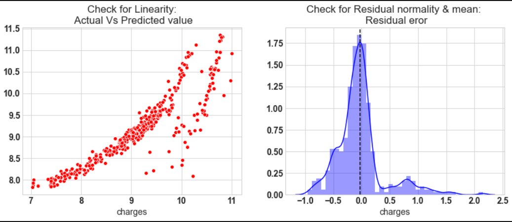
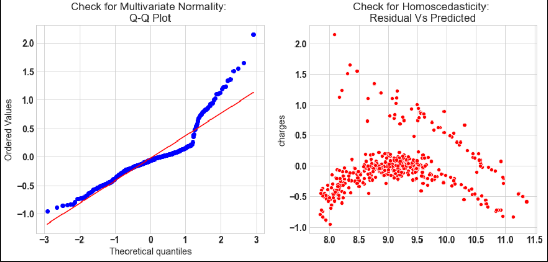
In order to validated model we need to check few assumption of linear regression model. The common assumption for Linear Regression model are following

1. Linear Relationship: In linear regression the relationship between the dependent and independent variable to be linear. This can be checked by scatter ploting Actual value Vs Predicted value
2. The residual error plot should be normally distributed.
3. The mean of residual error should be 0 or close to 0 as much as possible
4. The linear regression require all variables to be multivariate normal. This assumption can best checked with Q-Q plot.
5. Linear regession assumes that there is little or no *Multicollinearity in the data. Multicollinearity occurs when the independent variables are too highly correlated with each other. The variance inflation factor VIF identifies correlation between independent variables and strength of that correlation. , If VIF >1 & VIF <5 moderate correlation, VIF < 5 critical level of multicollinearity.
6. Homoscedasticity: The data are homoscedastic meaning the residuals are equal across the regression line. We can look at residual Vs fitted value scatter plot. If heteroscedastic plot would exhibit a funnel shape pattern.

The model assumption linear regression as follows

1. In our model the actual vs predicted plot is curve so linear assumption fails
2. The residual mean is zero and residual error plot right skewed
3. Q-Q plot shows as value log value greater than 1.5 trends to increase
4. The plot is exhibit heteroscedastic, error will insease after certian point.
5. Variance inflation factor value is less than 5, so no multicollearity.

Linearity plot and Residual plot.

Q-Q Plot and HomoScedasticity plot