Ensemble Models: Boosting Techniques

2021-02-04Blogs

Overview

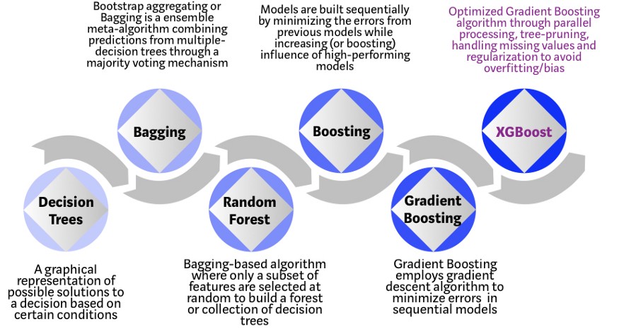
Boosting is a sequential process, where each subsequent model attempts to correct the errors of the previous model. The succeeding models are dependent on the previous model.
In this technique, learners are learned sequentially with early learners fitting simple models to the data and then analyzing data for errors. In other words, we fit consecutive trees (random sample) and at every step, the goal is to solve for net error from the prior tree.
When an input is misclassified by a hypothesis, its weight is increased so that next hypothesis is more likely to classify it correctly. By combining the whole set at the end converts weak learners into better performing model.
Let’s understand the way boosting works in the below steps.
1. A subset is created from the original dataset.
2. Initially, all data points are given equal weights.
3. A base model is created on this subset.
4. This model is used to make predictions on the whole dataset.
5. Errors are calculated using the actual values and predicted values.
6. The observations which are incorrectly predicted, are given higher weights. (Here, the three misclassified blue-plus points will be given higher weights)
7. Another model is created and predictions are made on the dataset. (This model tries to correct the errors from the previous model)
Thus, the boosting algorithm combines a number of weak learners to form a strong learner.
The individual models would not perform well on the entire dataset, but they work well for some part of the dataset.
Thus, each model actually boosts the performance of the ensemble.

We will discuss 3 major boosting models: AdaBoost, Gradient Boost and XGBoost.

AdaBoost

1. Definition

AdaBoost is an iterative ensemble method. AdaBoost classifier builds a strong classifier by combining multiple poorly performing classifiers so that you will get high accuracy strong classifier.
The basic concept behind Adaboost is to set the weights of classifiers and training the data sample in each iteration such that it ensures the accurate predictions of unusual observations.
Any machine learning algorithm can be used as base classifier if it accepts weights on the training set.
Stump: a tree with only 1 node and 2 leaves; Generally stumps does not perform as good as forest does; The AdaBoost uses the forest of stumps
AdaBoost should meet two conditions:
1. The classifier should be trained interactively on various weighed training examples.
2. In each iteration, it tries to provide an excellent fit for these examples by minimizing training error.
Complete Procedure
1. Assign each sample with a weight (initially set to equal weight) each row in Dataframe has a equal weight
2. Use the feature selection in decision node method to choose the first stump;
3. Measure how well a stump classifies the samples using: where is the weight of and is the set of misclassified datapoints
4. Determine the vote significance for the stump using
5. Laplace smoothing for the vote significance:
  in case Total Error = 1 or 0, the formula will return error, we add a small value in the formula
6. Modify the weight of samples so that next stump will take the errors that current stump made into account:
  6.1 Run each sample down the stump
  6.2 Compute new weight using:
  - Formula:
    - = New Sample Weight
    - = Current Sample weight.
    - = Amount of Say, alpha value, this is the coefficient that gets updated in each iteration and
    - = place holder for 1 if stump correctly classified, -1 if misclassified.
      6.3 Normalize the new weights
7. With the new sample weight we can either:
  - Use Weighted Gini Index to construct the next stump (Best feature for split)
  - Use a new set of sample derived from the previous sample:
    - pick until number of samples reach the size of original set
      - construct an interval-selection scheme using the sum of new sample weight as cutoff value if a number falls in i-th interval between (0,1), choose i-th sample;
        - e.g (0-0.07:1; 0.07-0.14:2; 0.14-0.60:3;0.60-0.67:4; etc)
      - randomly generate a number x between 0 and 1 pick the sample according to the scheme (note that the same sample can be repeatly picked)
8. Repeat Step 1 to 7 until the entire forest is built

2. Pros and Cons

Pros

Achieves higher performance than bagging when hyper-parameters tuned properly.
Can be used for classification and regression equally well.
Easily handles mixed data types.
Can use "robust" loss functions that make the model resistant to outliers.
AdaBoost is easy to implement.
We can use many base classifiers with AdaBoost.
AdaBoost is not prone to overfitting.

Cons

Difficult and time-consuming to properly tune hyper-parameters.
Cannot be parallelized like bagging (bad scalability when vast amounts of data).
More risk of overfitting compared to bagging.
AdaBoost is sensitive to noise data.
It is highly affected by outliers because it tries to fit each point perfectly.
Slower as compared to XGBoost

3. Comparison with Random Forest

Random Forest VS AdaBoost (Bagging vs Boosting)
- Random Forest uses full grown trees while Adaboost uses stumps (one root node with two leafs)
- In a Random Forest all the trees have similar amount of say, while in Adaboost some trees have more say than the other.
- In a random forest the order of the tree does not matter, while in Adaboost the order is important (especially since each tree is built by taking the error of the previous error).

4. Sample Code

import pandas as pd
import numpy as np
from sklearn.ensemble import AdaBoostClassifier
from sklearn.model_selection import train_test_split,GridSearchCV, StratifiedShuffleSplit
from sklearn.metrics import accuracy_score
from sklearn.preprocessing import StandardScaler


train = pd.read_pickle("train.pkl")

X = train.drop(['Survived'], axis = 1)
y = train["Survived"]

X_train, X_test, y_train, y_test = train_test_split(X, y, test_size = .33, random_state=0)

# Feature Scaling
## We will be using standardscaler to transform

st_scale = StandardScaler()

## transforming "train_x"
X_train = st_scale.fit_transform(X_train)
## transforming "test_x"
X_test = st_scale.transform(X_test)

adaBoost = AdaBoostClassifier(base_estimator=None,
                              learning_rate=1.0,
                              n_estimators=100)

adaBoost.fit(X_train, y_train)

y_pred = adaBoost.predict(X_test)


accuracy_score(y_test, y_pred)



n_estimators = [100,140,145,150,160, 170,175,180,185];
cv = StratifiedShuffleSplit(n_splits=10, test_size=.30, random_state=15)
learning_r = [0.1,1,0.01,0.5]

parameters = {'n_estimators':n_estimators,
              'learning_rate':learning_r
              
        }
grid = GridSearchCV(AdaBoostClassifier(base_estimator= None, ## If None, then the base estimator is a decision tree.
                                     ),
                                 param_grid=parameters,
                                 cv=cv,
                                 n_jobs = -1)
grid.fit(X,y) 

print (grid.best_score_)
print (grid.best_params_)
print (grid.best_estimator_)


adaBoost_grid = grid.best_estimator_
adaBoost_grid.score(X,y)

GBM (Gradient Boosting)

Gradient Boosting trains many models in a gradual, additive and sequential manner (sequential + homogeneous).
Major Motivation: allows one to optimise a user specified cost function, instead of a loss function that usually offers less control and does not essentially correspond with real world applications.
Main logic: utilizes the gradient descent to pinpoint the challenges in the learners' predictions used previously. The previous error is highlighted, and, by combining one weak learner to the next learner, the error is reduced significantly over time.
Procedure:

For Regression
1. Start by Compute the average of the , this is our 'initial prediction' for every sample
2. Then compute the ;
  - : Pseudo Residual at i-th sample
  - : True value of i-th sample
  - : Estimated value of i-th sample (here in first iteration)
3. Construct a new decision tree (fixed size) with the goal of predicting the residuals (a DT of , not the true value!!!)
4. If in a leaf, # of leaves < # of samples, then put the of samples that fall into same category into the same leaf; Then take average of all values on that leaf as output values;
5. Compute the new predicted value ()
  - : Newly Estimated value of i-th sample
  - : learning rate, usually between 0 ~ 0.1
  - : Estimated pseudo residual values (deduced from the decision tree)
6. Compute the new of each sample =
7. Construct the new tree with the new pseudo residual in step 5:
  - Repeat step 2, 3
  - Compute the new predicted value (here is deduced from a new DT):
  - Compute the new pseudo residual of each sample
8. Loop through the process UNTIL: adding additional trees does not significantly reduce the size of the pseudo residuals
For Classification
1. Set the initial prediction for every sample using ( is th probability of a sample being classified as 1)
  - : (same for every sample)
  - : log(odds) prediction for i-th sample, initially the same value, but value for each sample will change upon future iterations
  - Using logistic function for classification: ;
2. Decide on the classification: if > threshold, then "Yes"; else "No"; here the threshold may not be 0.5 (AUC and ROC to decide on the value);
3. Compute
4. Build a DT using the pseudo residual
5. Transformation of the pseudo residual to obtain the output values on each leaf:
  - e.g: if a leaf has (0.3, -0.7), then the leaf output value
6. Compute the new prediction
  - : log(odds) prediction for i-th sample in new iteration
  - : learning rate, usually between 0 ~ 0.1
7. Compute the new Probability
  - Compute the new predicted value for each sample;
  - Compute the new pseudo residual for each sample;
  - Build the new tree;
8. Loop until the pseudo residual does not change significantly;
Early Stopping: Early Stopping performs model optimisation by monitoring the model’s performance on a separate test data set and stopping the training procedure once the performance on the test data stops improving beyond a certain number of iterations.
- It avoids overfitting by attempting to automatically select the inflection point where performance on the test dataset starts to decrease while performance on the training dataset continues to improve as the model starts to overfit. In the context of gbm, early stopping can be based either on an out of bag sample set ("OOB") or cross- validation ("cv").

1. Pros & Cons

Pros

Robust against bias/outliers
GBM can be used to solve almost all objective function that we can write gradient out, some of which RF cannot resolve
Able to reduce bias and remove some extreme variances

Cons

More sensitive to overfitting if the data is noisy
GBDT training generally takes longer because of the fact that trees are built sequentially
Prone to overfitting, but can be overcame by parameter optimization

2. AdaBoost vs GBM

Both AdaBoost and Gradient Boosting build weak learners in a sequential fashion. Originally, AdaBoost was designed in such a way that at every step the sample distribution was adapted to put more weight on misclassified samples and less weight on correctly classified samples. The final prediction is a weighted average of all the weak learners, where more weight is placed on stronger learners.
Later, it was discovered that AdaBoost can also be expressed as in terms of the more general framework of additive models with a particular loss function (the exponential loss).
So, the main differences between AdaBoost and GBM are as follows:
1. The main difference therefore is that Gradient Boosting is a generic algorithm to find approximate solutions to the additive modeling problem, while AdaBoost can be seen as a special case with a particular loss function (Exponential loss function). Hence, gradient boosting is much more flexible.
2. AdaBoost can be interepted from a much more intuitive perspective and can be implemented without the reference to gradients by reweighting the training samples based on classifications from previous learners.
3. In Adaboost, shortcomings are identified by high-weight data points while in Gradient Boosting, shortcomings of existing weak learners are identified by gradients.
4. Adaboost is more about 'voting weights' and Gradient boosting is more about 'adding gradient optimization'.
5. Adaboost increases the accuracy by giving more weightage to the target which is misclassified by the model. At each iteration, Adaptive boosting algorithm changes the sample distribution by modifying the weights attached to each of the instances. It increases the weights of the wrongly predicted instances and decreases the ones of the correctly predicted instances.
6. AdaBoost use simple stumps as learners, while the fixed size trees of GBM are usually of maximum leaf number between 8 and 32;
7. Adaboost corrects its previous errors by tuning the weights for every incorrect observation in every iteration, but gradient boosting aims at fitting a new predictor in the residual errors committed by the preceding predictor.

3. Random Forest vs GBM

GBMs are harder to tune than RF. There are typically three parameters: number of trees, depth of trees and learning rate, and each tree built is generally shallow.
RF is harder to overfit than GBM.
RF runs in parallel while GBM runs in sequence

4. Application

A great application of GBM is anomaly detection in supervised learning settings where data is often highly unbalanced such as DNA sequences, credit card transactions or cybersecurity.

5. Sample Code implementation

import numpy as np
import pandas as pd
import matplotlib.pyplot as plt
from sklearn.preprocessing import MinMaxScaler
from sklearn.model_selection import train_test_split
from sklearn.ensemble import GradientBoostingClassifier
from sklearn.metrics import classification_report, confusion_matrix, roc_curve, auc


train = pd.read_csv("train.csv")
test = pd.read_csv("test.csv")

train.set_index("PassengerId", inplace=True)
test.set_index("PassengerId", inplace=True)

# generate training target set (y_train)
y_train = train["Survived"]
# delete column "Survived" from train set
train.drop(labels="Survived", axis=1, inplace=True)

train_test =  train.append(test)
# delete columns that are not used as features for training and prediction
columns_to_drop = ["Name", "Age", "SibSp", "Ticket", "Cabin", "Parch", "Embarked"]
train_test.drop(labels=columns_to_drop, axis=1, inplace=True)
# convert objects to numbers by pandas.get_dummies
train_test_dummies = pd.get_dummies(train_test, columns=["Sex"])

train_test_dummies.fillna(value=0.0, inplace=True)
# generate feature sets (X)
X_train = train_test_dummies.values[0:891]
X_test = train_test_dummies.values[891:]

scaler = MinMaxScaler()
X_train_scale = scaler.fit_transform(X_train)
X_test_scale = scaler.transform(X_test)

X_train_sub, X_validation_sub, y_train_sub, y_validation_sub = train_test_split(X_train_scale, y_train, random_state=0)

learning_rates = [0.05, 0.1, 0.25, 0.5, 0.75, 1]
for learning_rate in learning_rates:
    gb = GradientBoostingClassifier(n_estimators=20, learning_rate = learning_rate, max_features=2, max_depth = 2, random_state = 0)
    gb.fit(X_train_sub, y_train_sub)
    print("Learning rate: ", learning_rate)
    print("Accuracy score (training): {0:.3f}".format(gb.score(X_train_sub, y_train_sub)))
    print("Accuracy score (validation): {0:.3f}".format(gb.score(X_validation_sub, y_validation_sub)))
    print()
    
gb = GradientBoostingClassifier(n_estimators=20, learning_rate = 0.5, max_features=2, max_depth = 2, random_state = 0)
gb.fit(X_train_sub, y_train_sub)
predictions = gb.predict(X_validation_sub)

print("Confusion Matrix:")
print(confusion_matrix(y_validation_sub, predictions))
print()
print("Classification Report")
print(classification_report(y_validation_sub, predictions))

y_scores_gb = gb.decision_function(X_validation_sub)
fpr_gb, tpr_gb, _ = roc_curve(y_validation_sub, y_scores_gb)
roc_auc_gb = auc(fpr_gb, tpr_gb)

XGBoost

An optimized GBM
Evolution of XGBoost from Decision Tree
Procedure:

For Regression
1. Set initial value (by default is 0.5 [for both regression and classification])
2. Build the first XGBoost Tree (a unique type of regression tree):
  - Start with a root containing all the residuals ;
  - Compute similarity score where is the Regularization parameter.
  - Make a decision on spliting condition: For each consecutive samples, compute the mean k of 2 input as the threshold for decision node; then split by the condition feature_value < k
  - Decide the best thresold for spliting: Adopt the threshold that gives the largest Gain
  - For example: we have points {}:
    - Step 1: set the first threshold be
    - Step 2: now left node has {x1}, right node has {x2, x3}, we have and
    - Step 3: Compute
    - Step 4: Compute the second threshold and new Gain using this thresold
    - Step 5: Since gain of threshold 1 is greater than that of threshold 2, we use as the spliting threshold
  - If the leaf after spliting has > 1 residual, consider whether to split again (based on the residuals in the leaf);
  - continue until it reaches the max_depth (default is 6) or no more spliting is possible
  - Notes on
    1. A larger leads to greater likelihood of prunning as the are lower;
    2. The reduce the prediction’s sensitivity to nodes with low # of observations
3. Prune the Tree
  - From bottom branch up, decide on whether to prune the node/branch
    - : The threshold to determine if a Gain is large enough to be kept
    - if then prune (remove the branch);
    - Note that setting does not turn off prunnig!!!
  - If we prune every branch until it reaches the root, then remove the tree;
4. Compute
5. Compute New prediction
  - : Learning rate, default value = 0.3
  - : Output value of in each residual tree
6. Compute the new residuals for all samples, build the next tree and prune the tree;
7. Repeat the process just like Gradient Boost does; As more trees are built, the Gains will decease; We stop until the Gain < terminating value
For Classification
1. Set initial value (by default is 0.5)
2. Build the first XGBoost Tree:
  - Start with a root containing all the residuals
  - Compute similarity score where is the Regularization parameter.
  - Repeat the same procedure as the regression does; Compute all the Gains
  - Warning of Cover:
    - defined for the minimum number of residuals in each leaf (by default is 1)
    - in Regression: = # of Residuals in the leaf (always >= 1)
    - in Classification: = (not necessarily >= 1), hence some leafs violating the Cover threshold will be removed. Here Cover needs to be carefully chosen (like 0, 0.1, etc)
3. Prune the tree: same procedure as Regression case
4. Compute
5. Compute New prediction
  - : Learning rate, default value = 0.3
  - : Output value of in each residual tree (here is the first tree)
6. Convert into using logistic regression:
7. Compute the new residuals for all samples, build the next tree and prune the tree;
8. Repeat the process just like Gradient Boost does; As more trees are built, the Gains will decease; We stop until the Gain < terminating value;
9. Prediction:
  - ;

1. Advantage of XGBoost

Parallelized Tree Building
- Unlike GBM, XGBoost is able to build the sequential tree using a parallelized implementation
- This is possible due to the interchangeable nature of loops used for building base learners: the outer loop that enumerates the leaf nodes of a tree, and the second inner loop that calculates the features. This nesting of loops limits parallelization because without completing the inner loop (more computationally demanding of the two), the outer loop cannot be started. Therefore, to improve run time, the order of loops is interchanged using initialization through a global scan of all instances and sorting using parallel threads. This switch improves algorithmic performance by offsetting any parallelization overheads in computation.
Tree Pruning using depth-first approach
- The stopping criterion for tree splitting within GBM framework is greedy in nature and depends on the negative loss criterion at the point of split. XGBoost uses 'max_depth' parameter as specified instead of criterion first, and starts pruning trees backward. (This 'depth-first' approach improves computational performance significantly.)
Cache awareness and out-of-core computing
- allocating internal buffers in each thread to store gradient statistics. Further enhancements such as 'out-of-core' computing optimize available disk space while handling big data-frames that do not fit into memory.
Regularization
- It penalizes more complex models through both LASSO (L1) and Ridge (L2) regularization to prevent overfitting.
Efficient Handling of missing data
- XGboost decides at training time whether missing values go into the right or left node. It chooses which to minimise loss. If there are no missing values at training time, it defaults to sending any new missings to the right node.
In-built cross-validation capability
- The algorithm comes with built-in cross-validation method at each iteration, taking away the need to explicitly program this search and to specify the exact number of boosting iterations required in a single run.

LightGBM

A follow-up (and competitor) from XGBoost
Generally the same as GBM, except that a lot of optimizations are done, see this page to view all of them
Light GBM grows tree vertically while other algorithm grows trees horizontally meaning that Light GBM grows tree leaf-wise while other algorithm grows level-wise. It will choose the leaf with max delta loss to grow. When growing the same leaf, Leaf-wise algorithm can reduce more loss than a level-wise algorithm.
It is not advisable to use LGBM on small datasets. Light GBM is sensitive to overfitting and can easily overfit small data.

1. Advantages of Light GBM

Faster training speed and higher efficiency: Light GBM use histogram based algorithm i.e it buckets continuous feature values into discrete bins which fasten the training procedure.
Lower memory usage: Replaces continuous values to discrete bins which result in lower memory usage.
Better accuracy than any other boosting algorithm: It produces much more complex trees by following leaf wise split approach rather than a level-wise approach which is the main factor in achieving higher accuracy. However, it can sometimes lead to overfitting which can be avoided by setting the max_depth parameter.
Compatibility with Large Datasets: It is capable of performing equally good with large datasets with a significant reduction in training time as compared to XGBOOST.
Parallel learning supported

2. Code sample: XGBoost vs LightGBM

#importing standard libraries 
import numpy as np 
import pandas as pd 
from pandas import Series, DataFrame 

#import lightgbm and xgboost 
import lightgbm as lgb 
import xgboost as xgb 

#loading our training dataset 'adult.csv' with name 'data' using pandas 
data=pd.read_csv('adult.csv',header=None) 

#Assigning names to the columns 
data.columns=['age','workclass','fnlwgt','education','education-num','marital_Status','occupation','relationship','race','sex','capital_gain','capital_loss','hours_per_week','native_country','Income'] 

#glimpse of the dataset 
data.head() 

# Label Encoding our target variable 
from sklearn.preprocessing import LabelEncoder,OneHotEncoder
l=LabelEncoder() 
l.fit(data.Income) 

l.classes_ 
data.Income=Series(l.transform(data.Income))  #label encoding our target variable 
data.Income.value_counts() 

 

#One Hot Encoding of the Categorical features 
one_hot_workclass=pd.get_dummies(data.workclass) 
one_hot_education=pd.get_dummies(data.education) 
one_hot_marital_Status=pd.get_dummies(data.marital_Status) 
one_hot_occupation=pd.get_dummies(data.occupation)
one_hot_relationship=pd.get_dummies(data.relationship) 
one_hot_race=pd.get_dummies(data.race) 
one_hot_sex=pd.get_dummies(data.sex) 
one_hot_native_country=pd.get_dummies(data.native_country) 

#removing categorical features 
data.drop(['workclass','education','marital_Status','occupation','relationship','race','sex','native_country'],axis=1,inplace=True) 

 

#Merging one hot encoded features with our dataset 'data' 
data=pd.concat([data,one_hot_workclass,one_hot_education,one_hot_marital_Status,one_hot_occupation,one_hot_relationship,one_hot_race,one_hot_sex,one_hot_native_country],axis=1) 

#removing dulpicate columns 
_,i = np.unique(data.columns, return_index=True) 
data=data.iloc[:, i] 

#Here our target variable is 'Income' with values as 1 or 0.  
#Separating our data into features dataset x and our target dataset y 
x=data.drop('Income',axis=1) 
y=data.Income 

 

#Imputing missing values in our target variable 
y.fillna(y.mode()[0],inplace=True) 

#Now splitting our dataset into test and train 
from sklearn.model_selection import train_test_split 
x_train,x_test,y_train,y_test=train_test_split(x,y,test_size=.3)

#The data is stored in a DMatrix object 
#label is used to define our outcome variable
dtrain=xgb.DMatrix(x_train,label=y_train)
dtest=xgb.DMatrix(x_test)

#setting parameters for xgboost
parameters={'max_depth':7, 'eta':1, 'silent':1,'objective':'binary:logistic','eval_metric':'auc','learning_rate':.05}

#training our model 
num_round=50
from datetime import datetime 
start = datetime.now() 
xg=xgb.train(parameters,dtrain,num_round) 
stop = datetime.now()

#Execution time of the model 
execution_time_xgb = stop-start 
print(f'execution_time_xgb: {execution_time_xgb}')
#datetime.timedelta( , , ) representation $\implies$ (days , seconds , microseconds) 

#now predicting our model on test set 
ypred=xg.predict(dtest) 
display(ypred)

#Converting probabilities into 1 or 0  
for i in range(0, 9769): 
    if ypred[i] >= .5:
        ypred[i] = 1 
    else:
        ypred[i]=0  
        
#calculating accuracy of our model 
from sklearn.metrics import accuracy_score 
accuracy_xgb = accuracy_score(y_test,ypred) 
print(f'accuracy_xgb: {accuracy_xgb}')

train_data=lgb.Dataset(x_train,label=y_train)

#setting parameters for lightgbm
param = {'num_leaves':150, 'objective':'binary','max_depth':7,'learning_rate':.05,'max_bin':200}
param['metric'] = ['auc', 'binary_logloss']

#Here we have set max_depth in xgb and LightGBM to 7 to have a fair comparison between the two.

#training our model using light gbm
num_round=50
start=datetime.now()
lgbm=lgb.train(param,train_data,num_round)
stop=datetime.now()

#Execution time of the model
execution_time_lgbm = stop-start
print(f'execution_time_lgbm: {execution_time_lgbm}')

#predicting on test set
ypred2=lgbm.predict(x_test)
display(ypred2[0:5])  # showing first 5 predictions

#converting probabilities into 0 or 1
for i in range(0,9769):
    if ypred2[i]>=.5:       # setting threshold to .5
        ypred2[i]=1
    else:
        ypred2[i]=0
        
#calculating accuracy
accuracy_lgbm = accuracy_score(ypred2,y_test)
print(f'accuracy_lgbm: {accuracy_lgbm}')
display(y_test.value_counts())

from sklearn.metrics import roc_auc_score
#calculating roc_auc_score for xgboost
auc_xgb =  roc_auc_score(y_test,ypred)
print(f'auc_xgb: {auc_xgb}')

#calculating roc_auc_score for light gbm. 
auc_lgbm = roc_auc_score(y_test,ypred2)
print(f'auc_lgbm: {auc_lgbm}')
comparison_dict = {'accuracy score':(accuracy_lgbm, accuracy_xgb),'auc score':(auc_lgbm,auc_xgb),'execution time':(execution_time_lgbm, execution_time_xgb)}

#Creating a dataframe ‘comparison_df’ for comparing the performance of Lightgbm and xgb. 
comparison_df = DataFrame(comparison_dict) 
comparison_df.index= ['LightGBM','xgboost'] 
display(comparison_df)

3. General Pros and cons of boosting

Pros

Achieves higher performance than bagging when hyper-parameters tuned properly.
Can be used for classification and regression equally well.
Easily handles mixed data types.
Can use “robust” loss functions that make the model resistant to outliers.

Cons

Difficult and time consuming to properly tune hyper-parameters.
Cannot be parallelized like bagging (bad scalability when huge amounts of data).
More risk of overfitting compared to bagging.

Conclusion

Here we end the discussion about ensemble models. It was a fun and challenging topic. While most users of these model won't need to understand every nitty-gritty of these models, these profound theories laid significant foundations for future research on supervised ensemble learning models (and even meta-learning). In the next month, I'll share some posts about unsupervised learning. This is even large a topic, and I expect the content to be even deeper. Good luck, me and everyone!

Ensemble Models: Boosting Techniques

https://criss-wang.github.io/post/blogs/supervised/ensemble-2/

Author

Zhenlin Wang

Posted on

2021-02-04

Updated on

2021-10-11

Ensemble Models: Boosting Techniques

Overview

AdaBoost

1. Definition

2. Pros and Cons

3. Comparison with Random Forest

4. Sample Code

GBM (Gradient Boosting)

For Regression

For Classification

1. Pros & Cons

2. AdaBoost vs GBM

3. Random Forest vs GBM

4. Application

5. Sample Code implementation

XGBoost

For Regression

For Classification

1. Advantage of XGBoost

LightGBM

1. Advantages of Light GBM

2. Code sample: XGBoost vs LightGBM

3. General Pros and cons of boosting

Conclusion

Author

Posted on

Updated on

Licensed under

Tags

Catalogue