Variational Inference

Introduction

1. Background of Bayesian methods

In the field of machine learning, most would agree that frequentist approaches played a critical role in the development of early classical models. Nevertheless, we are witnessing the increasing significance of Bayesian methods in modern study of machine learning and data modelling. The simple-looking Bayes' rule has inspired a lot wonderful models in areas like topic modelling, representation learning and hyperparameter optimization. In these models, the latent variables are the focus of the study. By analysing several data on the observed variables , we hope to get some meaningful information (for example, a point estimate or an entire distribution) about these latent variables.

2. Problem with Bayesian methods: intractable integral

While the rule looks easily understandable, the numerical computation is hard in reality. One major issue is the intractable integral we need to compute in order to get the , which is often called the "model evidence". This is often because the search space for is combinatorially too large, making the computation extremely expensive. A common approach to deal with this problem is to approximate the posterior probability directly. Some popular choices include Monte Carlo Sampling methods and variational inference. In this report, we will introduce the variational methods, which are perhaps the most widely used inference technique in machine learning. We will analyse a particularly famous technique in variational methods, mean-field variational inference.

3. Main idea of variational inference

In variational inference, we can avoid computing the intractable integral by magically modelling the posterior directly. The main trick here is to approximate the unknown distribution with some similar distribution q. Since we can choose the q to belong to a certain family of distribution (hence tractable), the problem is now transformed into an optimization problem about the parameters of .

Understanding Variational Bayesian method

In this section, we demonstrate the theory behind variational Bayesian methods.

1. Kullback-Leibler Divergence

As mentioned above, variational inference needs a distribution to approximate the posterior distribution . Therefore we need to gauge how well a candidate approximates the posterior. A common measure is Kullback-Leibler Divergence (often called KL divergence).

KL divergence is defined as

Where means the expected value with respect to distribution . The formula can be interpreted as follows:

• if is low, the divergence is generally low.

• if is high and is high, the divergence is low.

• if is high and is low, the divergence is high, hence the approximation is not ideal.

Take note of the following about use of KL divergence in Variational Bayes:

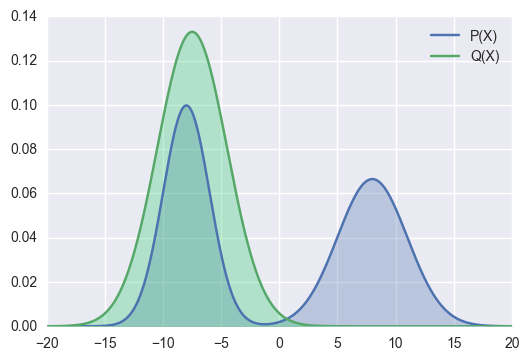
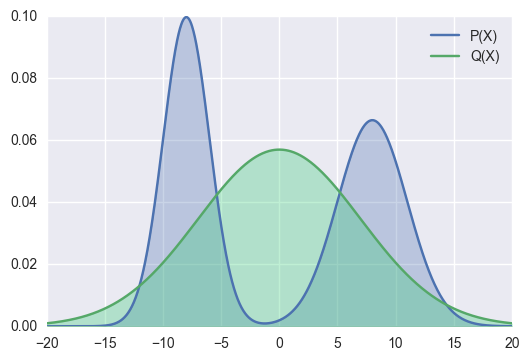
1. KL divergence is not symmetric, it's easy to see from the formula that as the approximation distribution is usually different from the target distribution .

2. In general, we focus on approximating some regions of as good as possible (Figure 1 (a)). It is not necessary for the to nicely approximate every part of As a result (usually called forward divergence) is not ideal. Because for some regions which we don't want to care, if , the KL divergence will be very large, forcing to take a different form even if it fits well with other regions of (refer to Figure 1(b)). On the other hand, (usually called reverse KL divergence) has the nice property that only regions where requires and to be similar. Consequently, reverse KL divergence is more commonly used in Variational Inference.

2. Evidence lower bound

Usually we don't directly minimizing KL divergence to obtain a good approximated distribution. This is because computing divergence still depends on the posterior . The computation involves the "evidence" term which is expensive to compute, as shown in the formula below:

The approximation using reverse KL divergence usually gives good empirical results, even though some regions of may be compromised

Figure 1: Reverse KL vs Forward KL divergence: The left image has a better approximation on part of . (a) Reverse KL simulation (b) Forward KL simulation

We can directly conclude by the fact that the term is than the log of evidence. We can also proof this result using Jensen's inequality as follows:

• By the definition of marginal probability, we have , take log on both side we have:

• The last 2 lines follow from Jensen's Inequality which states that for a convex function , we have

This term is known as the Evidence Lower Bound, or Since log does not depend on , we can treat it as a constant from the perspective of optimizing . Hence, minimizing is now equivalent to maximizing

General procedure

In general, a variational inference starts with a family of variational distribution (such as the mean-field family described below) as the candidate for . We can then use the manually chosen to compute the ELBO terms and . Afterwards, we optimize the parameters in to maximize the ELBO value using some optimization techniques (such as coordinate ascent and gradient methods).

Mean Field Variational Family

1. The "Mean Field" Assumptions

As shown above, the particular variational distribution family we use to approximate the posterior is chosen by ourselves. A popular choice is called the mean-field variational family. This family of distribution assumes joint approximation distribution to be factorized over some partition of the latent variables. This implies mutual independence among the n fractions in the partition. In particular: we have

where is factorized into . For simplicity, we assume that each fraction only contains 1 latent variable , it is often referred as "naive mean field". This family is nice to analyse because we can model each distribution with a tractable distribution based on the problem set-up. Do note that a limitation of this family is that we cannot easily capture the interdependence among the latent variables.

2. Derivation of optimal

Now in order to derive the the optimal form of distribution for and thus the overall , we need to go back to the ELBO optimization with this mean-field family assumption. Recall the formula for ELBO (we use here as it is the convention): We express this formula in terms of as using functional integral (see appendix A):

With this new expression, we can consider maximizing with respect to each of the . The optimal form of is the one which maximizes , that is:

We take the derivative with respect to using Lagrange multipliers and set to 0 yields:

where is a normalization constant that plays minimal role in the variable update.

The funtional derivative of this expression actually requires some knowledge about calculus of variations, specifically Euler-Lagrange equation.

3. Variable update with Coordinate Ascent

From equation we found that . Therefore iterative optimization algorithms like Coordinate Ascent can be applied to update the latent variables to reach their optimal form. Note that all the 's are interdependent during the update, hence in each iteration, we need to update all the 's. As short description for the coordinate ascent in this setup will be:

1. Compute values (if any) that can be directly obtained from data and constants

2. Initialize a particular to an arbitrary value

3. Update each variable with the step function

4. Repeat step 3 until the convergence of ELBO

A more detailed example of coordinate ascent will be shown in next section with the univariate gaussian distribution example. A point to take note that in general, we cannot guarantee the convexity of ELBO function. Hence, the convergence is usually to a local maximum.

Example with Univariate Gaussian

We demonstrate the mean-field variational inference with a simple case of observations from univariate Gaussian model. We first assume there are observations from a Gaussian distribution satisfying:

Here is inverse of variance (hence one-to-one correspondence). From the derivation of we know we need to compute the log joint probability . We will first derive an explicit formula for it by expanding the join probability into conditional probability:

where is a constant.

Note that sometimes some latent variable has higher priority that others. The choice of this variable depends on the exact question in hand.

1. Compute independent and

Next, we apply approximation via . By the mean-field assumption, we have . We proceed to find the optimal form of and :

• Compute the expression for :

Note that here is a shortcut representation for , and all are constant terms not involved in the optimization update. From the expression above, it's easy to observe that follows a Gaussian distribution with , where:

• Compute the expression for

A closer look at the result suggest that follows a Gaussian distribution with Gamma , where:

2. Variable update until ELBO convergence}

Now that we have and , we only need to update their parameters:

Using the updated and , we can then compute with Hence the coordinate ascent algorithm can be applied here:

1. Compute and as they can be derived directly from the data and constants based on their formula

2. Initialize to some random value

3. Update with current values of and

4. Update with current values of and

5. Compute ELBO value with the variables & updated with the parameters in step 1 - 4

6. Repeat the last 3 steps until ELBO value doesn't vary by much

As a result of the algorithm, we obtain an approximation for the posterior distribution of and given observations .

Extension and Further result

In this section, we briefly outline some more theory and reflection about general variational Bayesian methods. Due to space limitations, we only provide a short discussion on each of these.

Exponential family distributions in Varational Inference

A nice property of the exponential family distribution is the presence of conjugate priors in closed forms. This allows for less computationally intensive approaches when approximating posterior distributions (due to reasons like simpler optimization algorithm applicable and better analytical forms). Further more, Gharamani & Beal even suggested in 2000 that if all the belong to the same exponential family, the update of latent variables in the optimization procedure can be exact.

A great achievement in the field of variational inference is the generalized update formula for Exponentialfamily-conditional models. These models has conditional densities that are in exponential family. The nice property of exponential family leads to an amazing result that the optimal approximation form for posteriors are in the same exponential family as the conditional. This has benefits a lot of well-known models like Markov random field and Factorial Hidden Markov Model.

Comparison to other Inference methods

The ultimate results of variational inference are the approximation for the entire posterior distribution about the parameters and variables in the target problem with some observations instead of just a single point estimate. This serves the purpose of further statistical study of these latent variables, even if their true distributions are analytically intractable. Another group of inference methods commonly used to achieve the similar aim is Markov chain Monte Carlo (MCMC) methods like Gibbs sampling, which seeks to produce reliable resampling of given observations that help to approximate latent variables well. Another common Bayesian method that has a similar iterative variable update procedure is Expectation Maximization (EM). For EM, however, only point estimates of posterior distribution are obtained. The estimates are "Expectation maximizing" points, which means any information about the distribution around these points (or the parameters they estimate) are not preserved. On the other hand, despite the advantage of "entire distribution" Variational inference has, its point estimates are often derived just by the mean value of the approximated distributions. Such point estimates are often less significant compared to those derived using EM, as the optimum is not directly achieved from the Bayesian network itself, but the optimal distributions inferred from the network.

Popular algorithms applying variational inference

The popularity of variational inference has grown to even surpass the classical MCMC methods in recent years. It is particularly successful in generative modeling as a replacement for Gibbs sampling. The methods often show better empirical result than Gibbs sampling, and are thus more well-adopted. We here showcase some popular machine learning models and even deep learning models that heavily rely on variational inference methods and achieved great success:

• Latent Dirichlet Allocation: With the underlying Dirichlet distribution, the model applies both variational method (for latent variable distribution) and EM algorithm to obtain an optimal topic separation and categorization.

• variational autoencoder: The latent Gaussian space (a representation for the input with all the latent variables and parameters) is derived from observations, and fine-tuned to generate some convincing counterparts (a copy for instance) of the input.

These models often rely on a mixture of statistical learning theories, but variational inference is definitely one of the key function within them.