An overview of Hidden markov model and its algorithms

Overview

Stochastic Process is a critical piece of knowledge in statistical learning. It's also an important piece in the increasing popular reinforcement learning field. I feel like I might apply its algorithms or do research work on it in the future. Hence, I create this blog to introduce an important concept, hidden markov model (HMM), and some useful algorithms and their intuitions for HMM.

Markov Chain

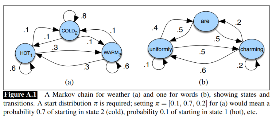
The HMM is based on augmenting the Markov Chain(MC), which is a type of a random process about a set of states. The transition from one state to another depends on certain probabilities , which we define as transition probability. The nice property of an MC is that the transition probability of only depends on the previous state , i.e. . We call it the Markov Assumption. This property allows us to produce an each transition graph like this^[1]
[1]:https://web.stanford.edu/~jurafsky/slp3/A.pdf

HMM Definition

A Markov chain is useful when we need to compute a probability for a sequence of observable events. In many cases, however, the events we are interested in are hidden: we don’t observe them directly. For example we don't normally observe part-of-speech tags in a text. Rather, we see words, and must infer the tags from the word sequence. We call the tags hidden because they are not observed. A hidden Markov model (HMM) allows us to talk about both observed events (like words that we see in the input) and hidden events (like part-of-speech tags) that we think of as causal factors in our probabilistic model. In HMM, we use observations to describe observed events with values denoted by , and states to describe hidden events with values denoted by . Note that Markov Assumption still holds. In addition, we have output independence . In HMM, we try to solve the following problems:

• Problem 1 (Likelihood): Given an HMM with transition probabilities and observation probabilities and an observation sequence , determine the likelihood .
• Problem 2 (Decoding): Given an observation sequence and an HMM , discover the best hidden state sequence .
• Problem 3 (Learning): Given an observation sequence and the set of states in the HMM, learn the HMM parameters and .

Algorithms

1. The Forward Algorithm - Likelihood solver

The forward algorithm is a dynamic programming method that computes the observation probability by summing over the probabilities of all possible hidden state paths that could generate the observation sequence, but it does so efficiently by implicitly folding each of these paths into a single forward trellis, which computes the probability of being in state after seeing the first observations, given the parameteres , i.e.

From above, we can quickly derive the result by:

1. first initialize .
2. Recrusively apply the above expression (1) for .
3. Compute

2. The Viterbi Algorithm - Decoding solver

Like forwarding algorithm, Viterbi is also DP that makes uses of a dynamic programming Viterbi trellis. The idea is to process the observation sequence left to right, filling out the trellis. Each cell of the trellis, , represents the probability that the HMM is in state after seeing the first observations and passing through the most probable state sequence , given the parameters . The value of each cell is computed by recursively taking the most probable path that could lead us to this cell.

Here, a major difference from (1) is that we now take the most probable of the extensions of the paths that lead to the current cell. In addition to the max value , we shall also keep track of the solution

This is called backpointers. We need this value because while the forward algorithm needs to produce an observation likelihood, the Viterbi algorithm must produce a probability and also the most likely state sequence. We compute this best state sequence by keeping track of the path of hidden states that led to each state, and Viterbi backtrace then at the end backtracing the best path to the beginning (the Viterbi backtrace).

Finally, we can compute the optimal score and path

We use a demo code to illustrate the process. The code for forwarding algorithm and Forward-Backward Algorithm can be implmented in a similar fashion.

import numpy as np
import pandas as pd

# Define the problem setup
obs_map = {'Cold':0, 'Hot':1}
obs = np.array([1,1,0,1,0,0,1,0,1,1,0,0,0,1])

inv_obs_map = dict((v,k) for k, v in obs_map.items())
obs_seq = [inv_obs_map[v] for v in list(obs)]

print("Simulated Observations:\n",pd.DataFrame(np.column_stack([obs, obs_seq]),columns=['Obs_code', 'Obs_seq']) )

pi = [0.6,0.4] # initial probabilities vector
states = ['Cold', 'Hot']
hidden_states = ['Snow', 'Rain', 'Sunshine']
pi = [0, 0.2, 0.8]
state_space = pd.Series(pi, index=hidden_states, name='states')
a_df = pd.DataFrame(columns=hidden_states, index=hidden_states)
a_df.loc[hidden_states[0]] = [0.3, 0.3, 0.4]
a_df.loc[hidden_states[1]] = [0.1, 0.45, 0.45]
a_df.loc[hidden_states[2]] = [0.2, 0.3, 0.5]
print("\n HMM matrix:\n", a_df)
a = a_df.values

observable_states = states
b_df = pd.DataFrame(columns=observable_states, index=hidden_states)
b_df.loc[hidden_states[0]] = [1,0]
b_df.loc[hidden_states[1]] = [0.8,0.2]
b_df.loc[hidden_states[2]] = [0.3,0.7]
print("\n Observable layer  matrix:\n",b_df)
b = b_df.values

# Apply the Viterbi Algorithm based on http://www.blackarbs.com/blog/introduction-hidden-markov-models-python-networkx-sklearn/2/9/2017
def viterbi(pi, a, b, obs):
    
    nStates = np.shape(b)[0]
    T = np.shape(obs)[0]
    
    # init blank path
    path = path = np.zeros(T,dtype=int)
    # delta --> highest probability of any path that reaches state i
    delta = np.zeros((nStates, T))
    # phi --> argmax by time step for each state
    phi = np.zeros((nStates, T))
    
    # init delta and phi 
    delta[:, 0] = pi * b[:, obs[0]]
    phi[:, 0] = 0

    print('\nStart Walk Forward\n')    
    # the forward algorithm extension
    for t in range(1, T):
        for s in range(nStates):
            delta[s, t] = np.max(delta[:, t-1] * a[:, s]) * b[s, obs[t]] 
            phi[s, t] = np.argmax(delta[:, t-1] * a[:, s])
            print('s={s} and t={t}: phi[{s}, {t}] = {phi}'.format(s=s, t=t, phi=phi[s, t]))
    
    # find optimal path
    print('-'*50)
    print('Start Backtrace\n')
    path[T-1] = np.argmax(delta[:, T-1])
    for t in range(T-2, -1, -1):
        path[t] = phi[path[t+1], [t+1]]
        print('path[{}] = {}'.format(t, path[t]))
        
    return path, delta, phi

# Run the algo
path, delta, phi = viterbi(pi, a, b, obs)
state_map = {0:'Snow', 1:'Rain', 2:'Sunshine'}
state_path = [state_map[v] for v in path]
pd.DataFrame().assign(Observation=obs_seq).assign(Best_Path=state_path)

3. Forward-backward algorithm - Learning solver

The standard algorithm for HMM training is the forward-backward, or Baum-Welch Welch algorithm, a special case of the Expectation-Maximization (EM) algorithm. The algorithm will let us train both the transition probabilities and the emission probabilities of the HMM. EM is an iterative algorithm, computing an initial estimate for the probabilities, then using those estimates to computing a better estimate, and so on, iteratively improving the probabilities that it learns.

For a real HMM, we only get observations, and cannot compute which observation is from which state directly from an observation sequence since we don't know which path of states was taken through the machine for a given input. What's more, we don't even know when is a hidden state present. The Baum-Welch algorithm solves this by iteratively estimating the number of times a state occurs. We will start with an estimate for the transition and observation probabilities and then use these estimated probabilities to derive better and better probabilities. And we're going to do this by computing the forward probability for an observation and then dividing that probability mass among all the different paths that contributed to this forward probability.

First, we define backward probability , the probability of seeing the observations from time to the end, given that we are in state at time (and given the automaton ):

We can actually think of it as a reverse of the forwarding probability , and the computation is just the "reverse" of that for , so now the computation of :

1. First initialize .
2. Recrusively apply .
3. Compute

Now, we start the actual work. To estimate the , we may adopt a simple maximum likelihood estimation

How do we compute the expected number of transitions from state to state ? Here's the intuition. Assume we had some estimate of the probability that a given transition was taken at a particular point in time in the observation sequence. If we knew this probability for each particular time , we could sum over all times to estimate the total count for the transition . We can then compute probability of being in state at time and state at time , given the observation sequence and of course the model via bayes' rule:

since we can easily compute

we get

Similarly, by considering expected number of times in state and observing symbol . Define the probability of being in state at time as , compute

We are ready to compute . For the numerator, we sum for all time steps in which the observation is the symbol that we are interested in. For the denominator, we sum over all time steps . The result is the percentage of the times that we were in state and saw symbol (the notation means “sum over all for which the observation at time was

Using (3), (4), we can apply EM algorithm easily, as demonstrated below:

• Initialize
• iterate until Convergence:

  • E-step:

    $$\xi_t(i, j) = \frac{\alpha_t(i) \widehat{P}_{ij} \widehat{P^H}j\left(o{t+1}\right) \beta_{t+1}(j)}{\sum_{j=1}^N \alpha_t(j) \beta_t(j)} \; \forall t, i \; \text{and} j
    $$

  • M-step:

This concludes the blog, thank you!