Model Validations and Performance Evaluators

Overview

Very often, people came up with various models with completely different underlying logics. In order to do reasonable comparisons among them, we must perform proper evaluations of the model performances and validate these models' efficacy via some datasets. This is where cross-validation comes in and performance metrics become extremely important. In this blog, I will first discuss about various techniques applied in cross-validation, followed by some analysis of commonly used metrics/scores

Cross validation

When we try to train a model, we require a training set and a test set. Very often, we need to split the training set itself so that we can use part of it as validation set: training proceeds on the training set, after which evaluation is done on the validation set, and when the experiment seems to be successful, final evaluation can be done on the test set. Unfortunately, this would be too wasteful of the dataset we have. To fully utilize our datasets, we need cross-validation, which can split our datasets in to folds, and we pick some folds as the choice for validation set. After several iterations ran with different choices, we take an average of the evaluation scores as the final performance score for the model.

The above strategy is often known as k-fold CV. It is computationally expensive, but it makes good use of the entire training set.

Cross Validation Methods

Based on the choice of folds we pick, we may end up with different CV methods. Below is a list of methods we can use and their intuitions:

1. Fixed index partition
   • K-Folds: partition the into k equal-sized subsets. choose 1 set from all subsets as the validation set. Run the model obtained only on this validation once.
   • Repeated K-Folds: run K-Folds n times, producing different splits and validation sets in each repetition.
2. Fixed validation set size
   • Leave One Out: Choose only one entry as the validation set
   • Leave P Out: Choose only entries as the validation set
3. Fixed label ratio
   • Stratified K-Folds: Each set contains approximately the same percentage of samples of each target class as the complete set.
4. Random index partition
   • Suffle & Split K-Folds: If we randomly pick entries in to get the resultant k partitioned subsets, we are equivalently doing shuffling before the partition.

All these data partition methods are very intuitive and can be found in sci-kit learn. Here I'll just give a demo of how code should be run for CV.

from sklearn.model_selection import cross_val_score
from sklearn.model_selection import ShuffleSplit
clf = svm.SVC(kernel='linear', C=1, random_state=42) # Some model here
cv = ShuffleSplit(n_splits=5, test_size=0.3, random_state=0) # You can specify the partition method here 
scores = cross_val_score(clf, X, y, cv=cv) # clf - model; X - training set; y - test set

Performance Metrics

Now let's move on to the next section on the metrics applied to evaluate the machine learning algorithms.

There are metrics used for different tasks:

• Supervised Classification
• Supervised Regression
• Unsupervised Clusetering

In this blog post, we will consider mainly on classification models, as the metrics for the remaining two task will be directly applied in these tasks to improve their model performances. We will leave it to interested readers to read my posts on models for these two tasks to explore the related metrics.

Classification

Note: Sometimes we have multiclass and multilabel problems instead of binary classifications. The answer from this post gives clear definitions for both problems:

Multiclass classification means a classification task with more than two classes; e.g., classify a set of images of fruits which may be oranges, apples, or pears. Multiclass classification makes the assumption that each sample is assigned to one and only one label: a fruit can be either an apple or a pear but not both at the same time.

Multilabel classification assigns to each sample a set of target labels. This can be thought of as predicting properties of a data-point that are not mutually exclusive, such as topics that are relevant for a document. A text might be about any of religion, politics, finance or education at the same time or none of these.

In the following discussions, I'll use [m-c] and [m-l] as labels to denote if the metric is applicable to Multiclass classification and Multilabel classification respectively.

1. Accuracy Score [m-l]

This is the ratio of number of correct predictions to the total number of input samples

• It works well only if there are equal number of samples belonging to each class. Otherwise, it may lead to over/under-estimation of the model's true performance due to imbalanced data.

2. Balanced accuracy score [m-c]

To address the problem above, we can introduce this score, which averages over recall scores per class where each sample is weighted according to the inverse prevalence of its true class.

• This formulation ensures that the score won't be too high just because one class's accuracy is high

3. Top-k accuracy score [m-l] [m-c]

A generalization of accuracy score: prediction is considered correct as long as the true label is associated with one of the k highest predicted scores.

4. Confusion Matrix [m-c]

The matrix which describes the complete performance of the model. This gives a good intuition over how well the classification is done. We can look at a sample pic here.¹

A sample confusion matrix

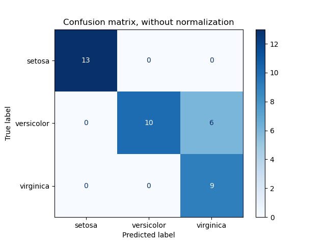
Based on the counts of corrected labeled and wrongly labeled samples, we can compute the following terms (say with regard to label 'sentosa', YES = is 'sentosa', NO = not 'sentosa')

• True Positives (TP) : The cases in which we predicted YES and the actual output was also YES.
• True Negatives (TN) : The cases in which we predicted NO and the actual output was NO.
• False Positives (FP) : The cases in which we predicted YES and the actual output was NO. Equivalently Type-I error.
• False Negatives (FN) : The cases in which we predicted NO and the actual output was YES. Equivalently Type-II error.

These four terms are crucial as they help to compute the following terms ¹:

• Precision: , intuitively the ability of the classifier not to label as positive a sample that is negative. It focuses on Type-I error.
• Recall: , intuitively the ability of the classifier to find all the positive samples. It focuses on Type-II error.
• F1-score: , a balanecd value (harmonic mean) of the precision and recall. We can generalize it to F-beta score, which allows more variated balanced between precision and recall:

5. Jaccard Similarity [m-l] [m-c]

The jaccard_score function computes the average of Jaccard similarity coefficients, also called the Jaccard index, between pairs of label sets.

6. Hinge Loss [m-c]

It only considers prediction errors. It is widely used in maximal margin classifiers such as support vector machines.
Suppose the label is in , output label is , true label is , then we have

7. Receiver operating characteristic (ROC) and Area Under Curve(AUC)

ROC is a plot of True Positive Rate (TPR)/Recall against False Positive Rates (FPR):

A sample image looks like this ¹:

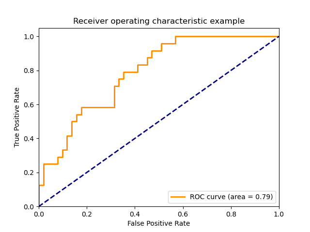
The area under the ROC curve is know as AUC, and it equals the probability that a randomly chosen positive example ranks above (is deemed to have a higher probability of being positive than negative) a randomly chosen negative example. The greater the value, the better is the performance.
Unfortunately, ROC curves aren't a good choice when your problem has a huge class imbalance.