MLOps Post Training Considerations

Introduction

Several years before, since I started working on ML projects, I've had traumatizing experiences conducting post-training operations. So many years later, I still found the mistakes and lessons I learnt from those projects valuable. Therefore, I've decided to share my thoughts here, for my own references (remember the do's and don'ts!!!) and for anyone interested to take their piece of gem home.

So what should be done after model training? Many university-level courses touched the surface of the topic, but in essence, it contains the handling of your model artifacts and training results, applying appropriate logging/monitoring and deployment to a server for actual usage. A great workflow chart I learned from Jeremy Jordan has demonstrated it well.

Credit: Jeremy Jordan

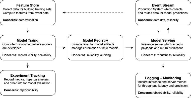
As you can see from the workflow:

• Experiment tracking is performed immediately after model training to persist the experiment results.
• Finetuned models are saved to a model registry (a form of database for model) to allow easy retrieval of this model
• Once we want to perform inference using this model, we set up a server which interacts with the registry and payload processed from backend to produce inference results
• A event stream (online or offline) service is need to enable drift detection and manage data flows. It should interact with inference server and your feature store actively, on a event-driven or scheduled manner
• Additional metric monitoring and backend logging are needed for issue recovery, model performance evaluation and reliability testing.

In this blog, I'll focus on experiment tracking, model registry, serving and monitoring. Note that I would not go through every detail in one blog, as you and I will both get tired reading a lengthy blog. I'll put some relevant links at places for people intereted to explore further. In the future, I'll also come up with blogs discussing each component in full detail as well. So stay tuned for that if you like my style XD.

Experiment Tracking

Every mature data scientist and ml engineer/researcher should appreciate the important of experiment tracking:

• Reproducibility: ML experiments often involve multiple dependencies and configurations. Tracking every experiment ensures reproducibility, allowing researchers to revisit and replicate results.
• Collaboration: In team environments, multiple researchers may contribute to a project. Clear experiment tracking facilitates collaboration by providing a shared understanding of the progress and results.
• Model Iteration: Continuous improvement is a core aspect of deep learning. Experiment tracking helps monitor model iterations, enabling researchers to identify what works and what doesn't.

There are a few components in experiment tracking:

1. Logging: Maintain a log for each experiment and save it in a unified place. Log your model hyperparameters, experiment metrics, and any other relevant information. This aids in easy retrieval and comparison.
2. Version Control: this include tagging and versioning of your training data, your model, metadata and experiments. This significantly reduces the chance of redoing experiments which may result in significant waste of resources (Yes I did this once…)
3. Metadata Annotation: Annotate experiments with metadata such as project name, researcher name, and experiment purpose. This contextual information proves invaluable in understanding the context of each experiment.
4. Visualization: Use visualization tools to track and compare metrics across experiments. This aids in identifying trends, outliers, and areas for improvement. In many cases, inputs and outputs stored are visualized as well.

Platforms to use

Nowadays, tracking experiments are much easier than 5, 10 years ago with the help of well-developed tracking tools. A few powerful ones I've used and would recommend are

• MLflow
• Weights & Biases (WandB)
• Neptune.ai

These tools have api's directly embedded in your training scripts. For example, for mlflow, all you need to do is run mlflow ui

import mlflow

experiment_name = "YOUR_EXPERIMENT_NAME"
run_name = datetime.now().strftime("%Y%m%d-%H%M")
mlflow.set_tracking_url("http://localhost:5000") # replace it if you have a dedicated tracking server url
mlflow.set_experiment(experiment_name=experiment_name)

with mlflow.start_run(experiment_id=experiment_id, run_name=run_name):
    # Start your model training
    ...
    # logging metrics
    metrics = YOUR_METRICS_GETTER
    mlflow.log_metric(...)

    # logging artifact
    mlflow.log_artifact(...)

and you will get a beautiful ui that looks like this:

Tracking individual components

Tracking Errors

To enable logging errors, one can use the default python logger, and save the log history as text/artifacts into these platforms. Otherwise, tools like WandB also has its integrated logger that directs the std outputs into its db and saves the log conveniently.

Tracking Hyperparameters

• Method 1: config yaml file
  in a yaml file

project: ORGANIZATION/home-credit
name: home-credit-default-risk

parameters:
  # Data preparation
  n_cv_splits: 5
  validation_size: 0.2
  stratified_cv: True
  shuffle: 1

  # Random forest
  rf__n_estimators: 2000
  rf__criterion: gini
  rf__max_features: 0.2
  rf__max_depth: 40
  rf__min_samples_split: 50
  rf__min_samples_leaf: 20
  rf__max_leaf_nodes: 60
  rf__class_weight: balanced

  # Post Processing
  aggregation_method: rank_mean

then in your python file you can do:

import yaml

with open(config_path) as f:
	# note that you should choose loader wisely as some values (e.g. int) may be parsed wrongly if you use the wrong loader
    config = yaml.load(f, Loader=yaml.SafeLoader)  # config is dict

print(config['parameters']['n_cv_splits'])  # 5

• Method 2: command line + argparse
  The most common choice in ML community (and the most convoluted one)

• Method 3: Hydra
  using the same yaml file, do the folloing

import hydra
from omegaconf import DictConfig

@hydra.main(config_path='hydra-config.yaml')
def train(cfg):
    print(cfg.pretty())  # this prints config in a reader friendly way
    print(cfg.parameters.rf__n_estimators)  # this is how to access single value from the config
if __name__ == "__main__":
    train()

Tracking Data

Ensure your data source is coherent and versioned consistently requires the use of data registry sometimes. One example is using DVC. You may refer to this AWS Tutorial on DVC usage to setup your data registry. Due to the versatile nature of data sources, we cannot always rely on a SQL DB (e.g. MySQL) or NoSQL DB (e.g MongoDB, InfluxDB) to manage our experiment training data, hence the usage of DVC.

Tracking Metrics

Normally metrics are easily to track directly with the tools I mentioned above. Very often they come with the set of visualizations as well. In case you need to produce your own visualizations, especially when evaluting the impact of model configurations on the metric values, libraries like optuna, hyperopt and scikit-optimize will have support for visualizations.

Tracking Model Environment

• Solution 1: Docker images (preferred)
• Create a Dockerfile

# Use a miniconda3 as base image
FROM continuumio/miniconda3

# Installation of jupyterlab
RUN pip install jupyterlab==0.35.6 &&
pip install jupyterlab-server==0.2.0 &&
conda install -c conda-forge nodejs

# Installation of Neptune and enabling neptune extension
RUN pip install neptune &&
pip install neptune-notebooks &&
jupyter labextension install neptune-notebooks

# Setting up Neptune API token as env variable
ARG NEPTUNE_API_TOKEN
ENV NEPTUNE_API_TOKEN=$NEPTUNE_API_TOKEN

# Adding current directory to container
ADD . /mnt/workdir
WORKDIR /mnt/workdir

• run docker build -t YOUR_TAG --build-arg NEPTUNE_API_TOKEN=$NEPTUNE_API_TOKEN .
• finally start the image by (example below)

docker run
    -p 8888:8888
    IMAGE_TAG:latest
    /opt/conda/bin/jupyter lab
    --allow-root
    --ip=0.0.0.0
    --port=8888

• Solution 2: conda
  • Usually  .yaml configuration file
  • create conda environment by running: conda env create -f environment.yaml
  • update yaml fle by conda env export > environment.yaml

Tracking Models

Model needs to be versioned and the artifacts stored in model registry, which I'll talk about in the next section.

Model Registry

Saving and versioning a model can be done at experiment tracking stage, or isolated out as a single stage in the workflow. This is because we usually have it as an output of the experiment runs, and it involves several more intricate details. A few aspects include:

• Different environment the registry (dev/stage/prod)
• Different forms of registering models (save/package/store)

Dev vs Prod Registry

• Purpose:
  • Dev Environment: where data scientists and machine learning engineers work on creating, experimenting, and refining
    • rapid iterations
    • multiple experiments
    • exploratory models
  • Prod Environment: where the finalized, stable, and optimized models are deployed to serve predictions in a real-world setting. Production models are expected to be reliable, scalable, and performant
    • mainly consist of champion models and challenger models
    • both should be well-tested and verified before saved in this registry
• Access and Permissions:
  • Dev Environment: access might be more open to facilitate collaboration and experimentation.
    • Data scientists/MLEs often have broader access to try out different ideas and approaches.
  • Prod Environment: access to the model registry in the production environment is typically more restricted
    • Authorized personnel, such as DevOps or IT administrators, should have the ability to deploy or update models in the production registry to maintain stability and security
    • Less of a concern from data scientist perspective
• Model Versions:
  • Dev Environment: usually a large number of model versions as different experiments and iterations are conducted.
  • Prod Environment: have fewer, well-tested, and validated model versions. The focus is on deploying stable models that meet performance and reliability requirements.
• Logging and Monitoring:
  • Dev Environment: more focused on tracking experiment results, understanding model behavior, and debugging
  • Prod Environment: critical for tracking the performance of deployed models, identifying issues in real-time, and ensuring that the system meets service-level objectives.
• Security Considerations:
  • Dev Environment: Security measures in the development environment may be more relaxed to enable faster experimentation
    • Model is within internal control, less exposed to external uses.
    • Major concern is actually training/testing data leakage
  • Prod Environment: Strict security measures are implemented in the production environment to safeguard against unauthorized access, data breaches, or other security threats
    • Prevent leakage of model information (metadata, weights, architectures, etc) as they are important company properties

Save vs package vs store ML models

1. Save Model
   • Save params to disk
   • Mainly for local operations on a single model(save/load model state dict, optim state dict, etc)
   • Tools: Pickle, HDFS, JSON, etc
2. Package Model
   • Bundle model with additional resources (model file, dependencies, configuration files, etc)
   • Enable easy distribute and deploy the ML model in a production environment
   • Tools: Docker Image, Python Packages
3. Store Model
   • Mainly for centralized model storage (model artifact)
   • To facilitate model sharing across team
   • Tools: MLFlow

Save

import torch

# Load the model and optimizer
model = ...
optimizer = ...

# Save the model and optimizer states in a single file
torch.save(
	{'model': model.state_dict(),
	 'optimizer': optimizer.state_dict()}, 'saved_states.pt')

# Load the saved states from the file
saved_states = torch.load('saved_states.pt')

# Restore the model and optimizer states from the dictionary
model.load_state_dict(saved_states['model'])
optimizer.load_state_dict(saved_states['optimizer'])

Package

# load dependencies
import onnx
import onnxruntime


# Load your trained model (e.g., PyTorch or TensorFlow)
model = ...

# Convert the model to ONNX format
onnx_model = onnx.convert(model, 'my_model')

# Save the ONNX model to a file
with open('my_model.onnx', 'wb') as f:
    f.write(onnx_model.SerializeToString())

# Load the ONNX model from the file
onnx_model = onnx.load('my_model.onnx')

# Create a new session for the model
session = onnxruntime.InferenceSession(onnx_model)

# Use the session to perform inference or deployment
inputs = ...  # Get input data (e.g., images, audio samples, etc.)
outputs = session.run(None, inputs)

Store

• Either use Database to store model versions, or consider using a model registry
• Example of MLFlow

import mlflow

# Load your trained model (e.g., PyTorch or TensorFlow)
model = ...

# Create a new experiment for the model in the Model Registry
experiment_id =
mlflow.get_experiment(experiment_name="MyModelExperiment").experiment_id

# Set up the artifact for the model
artifact_path = "models/my_model"
artifact_uri = f"runs:/{experiment_id}/{artifact_path}"

# Log the artifact to the Model Registry
mlflow.log_artifact(model, artifact_uri)

Model Serving

Model serving is actually a fairly complicated process, as it involves deep understanding of backend engineering and data engineering, as well as more infrastructure management. There are several methods to serve/deploy a model:

• Online
• Offline
• Streaming
• Batch
• Serverless

For the simplest part, all you'll need is to parse the data from the request, feed it as input (after feature engineering) into the model you loaded, and get the result. However, in order to make model serving efficient and powerful, many parts of the process need to be optimized:

API architecture

A few strong candidates to build the request/response formatting for data communication when deploying model are Remote Procedure Call (RPC), WebSocket, and RESTful APIs. Let's discuss the trade-offs associated with each approach:

1. Remote Procedure Call (RPC):

• Pros:
  • Efficiency: RPC protocols (e.g., gRPC) are known for their efficiency, making them suitable for scenarios where low-latency communication is crucial.
  • Streaming: Some RPC frameworks support bidirectional streaming, allowing continuous communication between clients and servers, which can be beneficial for real-time updates.
• Cons:
  • Complexity: Implementing and managing RPC services can be more complex than other approaches, especially when dealing with advanced features like bidirectional streaming.

2. WebSocket:

• Pros:
  • Low Latency: WebSockets provide low-latency, full-duplex communication, making them suitable for applications requiring real-time updates.
  • Bidirectional Communication: WebSockets enable bidirectional communication, allowing the server to push updates to clients efficiently.
• Cons:
  • Connection Management: Managing WebSocket connections can be more challenging than REST APIs, especially when dealing with issues like connection drops and reconnections.
  • Standardization: WebSockets lack a standardized way to describe APIs compared to RESTful APIs.

3. RESTful API:

• Pros:
  • Simplicity: RESTful APIs are simple and easy to understand, making them accessible to a wide range of developers.
  • Widespread Adoption: RESTful APIs are widely adopted and supported by a vast ecosystem of tools and libraries.
    Statelessness: RESTful APIs are inherently stateless, simplifying scalability and fault tolerance.
• Cons:
  • Latency: For real-time applications, RESTful APIs might introduce higher latency due to the request-response nature of communication.
  • Limited Push Mechanism: Traditional REST APIs lack a built-in mechanism for the server to push updates to clients in real-time.

Online vs Offline

Notice that while some part of the inference may require online models, other parts of the system may be done offline. Take a recommendation system for example:

• The latest recommended feeds should be generated in real-time/online. However, some of the embedding/coarse search may be done offline in fixed duration. The results of these offline inferences are then used as embeddings/context for the refined search/ranking during the real-time inference stage.

ETL-based Deployment

ETL (Extract, Transform, Load) jobs copy and process data from a source to a destination, commonly used in data warehousing. In machine learning model deployment, ETL involves extracting features, predicting, and saving results. Unlike real-time systems, ETL jobs don't provide quick predictions but process many records at once, contrasting with web apps. You may use ETL structure for serving the model when your app is monolith and the pipeline is less convoluted. Tools like Apache Beam, MapReduce or Airflow are perfect tools for performing ETL-driven model serving.

Model service as part of Microservices

If you are serving model on a larger distributed system with many microservices, you would likely need to consider inter-service communication, and push your inference task into an event queue if necessary. Tools like Kafka, RabbitMQ and Celery are designed to achieve this by ways of pub-sub or message brokers. Further discussion will cause it to divert into the field of backend system design, and I shall stop here for interested people to learn more on themselves.

Serverless Architecture

If you don't want to setup a server yourself (managing the infra can be a huge pain) and would like an endpoint that is fault-tolerant, scalable and ready-to-use, many cloud service companies have it available. Examples include Azure ML, AWS Lambda and GCP AI Studio. You can find tutorials on respective tools to setup your inference endpoint with the model you've developed.

Model Monitoring

Metrics to monitor

Model metrics

• Prediction distributions
• Feature distributions
• Evaluation metrics (when ground truth is available)

System metrics

• Request throughput
• Error rate
• Request latencies
• Request body size
• Response body size

Resource metrics

• CPU utilization
• Memory utilization
• Network data transfer
• Disk I/O

Sample procedure for ML app monitoring

1. Create a containerized REST service to expose the model via a prediction endpoint.

2. Setup Instrumentor to collect metrics which are exposed via a separate metrics endpoint

   • In the repo from JJ, it is instrumentator.instrument(app).expose(app, include_in_schema=False, should_gzip=True)
   • After deploying our model service on the Kubernetes cluster, we can port forward to a pod running the server and check out the metrics endpoint running at 127.0.0.1:3000/metrics:
   • kubectl port-forward service/wine-quality-model-service 3000:80

3. Deploy Prometheus (PULL-based mechanism) to collect and store metrics.

   • Prometheus refers to endpoints containing metric data as targets which can be discovered either through service discovery or static configuration.
   • Usually service discovery would be a good choice as it enable Prometheus to discover which targets should be scraped
   • This can be simply done by configuring the endpoints to monitor in a separate service

   ---
   endpoints:
     - path: metrics
       port: app
       interval: 15s

4. Deploy Grafana to visualize the collected metrics.

5. Finally, we'll simulate production traffic using Locust so that we have some data to see in our dashboards. Some of the standard tests to include are:

   1. Make a request to our health check endpoint
   2. choose a random example from the dataset and make a request to prediction service
   3. choose a random example, corrupt the data, and make a bad request to our prediction service

Other things to consider

1. Drift Detection Service
   • Strategies
     • deploy a drift-detection service
     • log a statistical profile
     • log the full feature payload
   • 

Best Practices

Prometheus

• Avoid storing high-cardinality data in labels. Every unique set of labels for is treated as a distinct time series, high-cardinality data in labels can drastically increase the amount of data being stored. As a general rule, try to keep the cardinality for a given metric (number of unique label-sets) under 10.
• Metric names should have a suffix describing the unit (e.g. http_request_duration_****seconds****)
• Use base units when recording values (e.g. seconds instead of milliseconds).
• Use standard Prometheus exporters when available.

Grafana

• Ensure your dashboards are easily discoverable and consistent by design.
• Use template variables instead of hardcoding values or duplicating charts.
• Provide appropriate context next to important charts.
• Keep your dashboards in source control.
• Avoid duplicating dashboards.

https://towardsdatascience.com/testing-features-with-pytest-82765a13a0e7

Last words

While this blog covers a lot of topics and provide several examples in the processing of post-training tasks, they are far to complete. In order to truly master each component, I would recommend play around with each part for a few times and make mistakes. This was the path I took, but without any preliminary guide like this. Nonetheless, it was fruitful and really helped me understand the nitty gritty of post-training tasks. Hence, review this blog when you feel like setting up a new project, and make it part of the process!