The Data Mining Triology: II. Cleaning

Overview

Very often, the data loaded into your notebooks are not entirely usable. There might be missing values, noisy data points, duplicates and outliers. Sometimes, data needs to be scaled up and down. Encoding and dimensionality reductions can be performed to make data cleaner and easier to operate on. Here we discuss about some essential ways to clean up the data

Basic Cleaning

The first step involves

1. Detecting and handling missing or noisy data;
2. Removal of outliers
3. Minimizing duplication and computed biases within the data

---

• Missing Data

  Missing data is the entries with empty input or Null input. It can be handled in following ways:

  1. Ignore the Tuple

     Note: Suitable only when the dataset is quite large and multiple values are missing within a tuple

  df2 = df[[column for column in df if df[column].count() / len(df) >= 0.3]] # Drops columns with >70% of rows missing value;
  
  print("List of dropped columns:", end=" ")
  for c in df.columns:
  	if c not in df2.columns:
  		print(c, end=", ") # list out the dropped columns

  2. Fill the Missing Values using
     • Manual imputation (via inspection & domain knowledge)
     • Mean value imputation
     • Most Probable Value (Mode) imputation

• Noisy Data

  Noisy data is meaningless data that can't be interpreted by machines. It can be generated due to faulty data collection, data entry errors etc. It can be handled in following ways :

  1. Binning Method:

     [Sorted data in order to smooth it] [The whole data divided into segments of equal size] [Various methods are performed to complete the task. Each segmented is handled separately.]

  2. Regression:

     Fitting data to a regression function: ML Regression Algorithm can be used for smoothing of data. Interpolate using the regression.

  3. Clustering:

  Groups the similar data in a cluster and apply unsupervised learning.

• Detect and Remove Outliers:

  • Detect Outliers (Some simple methods outlined below)

  1. Using Boxplot

  import seaborn as sns
  sns.boxplot(...)

  2. Using Scatterplot

  %matplotlib inline
  from matplotlib import pyplot as plt
  fig, ax = plt.subplots(figsize=(16,8))
  ax.scatter(...)
  plot.show()

  3. Using z score

  from scipy import stats
  import numpy as np
  z = np.abs(stats.zscore(boston_df))
  threshold = 3
  print(np.where(z > threshold))

  4. Using interquartile range (IQR) score

  Q1 = boston_df_o1.quantile(0.25)
  Q3 = boston_df_o1.quantile(0.75)
  IQR = Q3 - Q1
  print(boston_df_o1 < (Q1 - 1.5 * IQR)) |(boston_df_o1 > (Q3 + 1.5 * IQR))

  • Remove Outliers (Fixed value or interval methods)

  5. Using column specific value threshold

  boston_df_o = boston_df_o[(z < 3).all(axis=1)]

  6. Using value range (IQR in this case)

  boston_df_out = boston_df_o1[~((boston_df_o1 < (Q1 - 1.5 * IQR)) |(boston_df_o1 > (Q3 + 1.5 * IQR))).any(axis=1)]

• Remove Duplicates

  Sometimes, there may exist duplicate data entries. Most of the time, this is undesirable. You may want to remove those entries (after carefully examine the problem setups)

   s1_dup = s1_trans[s1_trans.duplicated()] # Identify Duplicates
  print(s1_dup.shape)
  s1_trans.drop_duplicates(subset = None, keep = 'first', inplace = True) # Remove Duplicates

Transforming data

We transform datasets in some situations to :

1. Convert the raw data into a specified format according to the need of the model.
2. Remove redundancy within the data (not duplicates, but unnecessary bytes that occupy the storage for no meaning)
3. Efficiently organize the data

Here we just present the method using sci-kit laern's preprocessing module.

Data Conversion

1. Normalization (Basically Data rescaling/mean removal):
   It is done in order to scale the data values in a specified range (-1.0 to 1.0 or 0.0 to 1.0)

2. Attribute Selection (Usually for Aggregation purpose):
   In this strategy, new attributes are constructed from the given set of attributes to help the mining process.

3. Discretization: (IMPT!!!)
   This is done to replace the raw values of numeric attribute by interval levels or conceptual levels.

   • Using classes/ranges/bands mapping (given or need to design)
   • Using Top-down approaches: Entropy-based Discretization

4. Concept Hierarchy Generation:
   Here attributes are converted from level to higher level in hierarchy. For example, the attribute "city" can be converted to "country" in some scenarios.

5. Encode Data:
   Machine learning algorithms cannot work with categorical data directly, categorical data must be converted to number.

   1. Label Encoding
   2. One hot encoding
   3. Dummy variable trap

   Label encoding refers to transforming the word labels into numerical form so that the algorithms can understand how to operate on them.

   A One hot encoding is a representation of categorical variable as binary vectors.It allows the representation of categorical data to be more expresive. This first requires that the categorical values be mapped to integer values, that is label encoding. Then, each integer value is represented as a binary vector that is all zero values except the index of the integer, which is marked with a 1.

   The Dummy variable trap is a scenario in which the independent variable are multicollinear, a scenario in which two or more variables are highly correlated in simple term one variable can be predicted from the others.

   By using pandas get_dummies function we can do all above three step in line of code. We will this fuction to get dummy variable for sex, children,smoker,region features. By setting drop_first =True function will remove dummy variable trap by droping one variable and original variable.The pandas makes our life easy.

6. Advanced: Box-Cox transformation
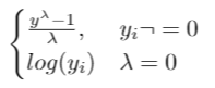
   A Box Cox transformation is a way to transform non-normal dependent variables into a normal shape. Normality is an important assumption for many statistical techniques; if your data isn't normal, applying a Box-Cox means that you are able to run a broader number of tests. All that we need to perform this transformation is to find lambda value and apply the rule shown below to your variable.

   ## The trick of Box-Cox transformation is to find lambda value, however in practice this is quite affordable. The following function returns the transformed variable, lambda value,confidence interval. See the sample code below:
   from scipy.stats import boxcox
   y_bc,lam, ci= boxcox(df_encode['charges'],alpha=0.05) 

box-cox

Data Scaling / Standardizing / Mean Removal

Note: Don't use all of them, only use some selectively when you need to (which is usually the case after EDA)!!!

1. Rescaling Data: scaled between the given range

   data_scaler = preprocessing.MinMaxScaler(feature_range = (0, 1))
   data_scaled = data_scaler.fit_transform(input_data)

2. Mean Removal: standardize input_data into mean = 0 and std = 1

   data_standardized = preprocessing.scale(input_data)
   data_standardized.mean(axis = 0)
   data_standardized.std(axis = 0)

3. Normalizing Data: values of a feature vector are adjusted so that they sum up to 1

   data_normalized = preprocessing.normalize(input_data, norm  = 'l1')

4. Binarizing Data: convert a numerical feature vector into a Boolean vector

   data_binarized = preprocessing.Binarizer(threshold=1.4).transform(input_data)

5. Label Encoding: changing the word labels into numbers

   ### Encode:
   label_encoder = preprocessing.LabelEncoder()
   input_classes = ['suzuki', 'ford', 'suzuki', 'toyota', 'ford', 'bmw']
   label_encoder.fit(input_classes) #Generate Mapping
   print("\nClass mapping:")
   for i, item in enumerate(label_encoder.classes_):
     print(item, '-->', i)
   labels = ['toyota', 'ford', 'suzuki']
   encoded_labels = label_encoder.transform(labels) # Actual Encoding
   ### Decode:
   decoded_labels = label_encoder.inverse_transform(encoded_labels) # Actual Decoding

   Warning: it assumes higher the categorical value, better the category (solved by one hot encoding)
6. One Hot Encoding (often used together with argmax function): Dummy Variable Encoding

   >>> enc = OneHotEncoder(handle_unknown='ignore')
   >>> X = [['Male', 1], ['Female', 3], ['Female', 2]]
   >>> enc.fit(X)
   OneHotEncoder(handle_unknown='ignore')
   >>> enc.categories_
   [array(['Female', 'Male'], dtype=object), array([1, 2, 3], dtype=object)]
   >>> enc.transform([['Female', 1], ['Male', 4]]).toarray()
   array([[1., 0., 1., 0., 0.],
         [0., 1., 0., 0., 0.]])
   >>> enc.inverse_transform([[0, 1, 1, 0, 0], [0, 0, 0, 1, 0]])
   array([['Male', 1],
         [None, 2]], dtype=object)

7. Scaler Comparison and choices
   1. MinMaxScaler
      • Definition: Add or substract a constant. Then multiply or divide by another constant. MinMaxScaler subtracts the mimimum value in the column and then divides by the difference between the original maximum and original minimum.
      • Preprocessing Type: Scale
      • Range: 0 to 1 default, can override
      • Mean: varies
      • Distribution Characteristics: Bounded
      • When Use: Use first unless have theoretical reason to need stronger scalers.
      • Notes: Preserves the shape of the original distribution. Doesn't reduce the importance of outliers. Least disruptive to the information in the original data. Default range for MinMaxScaler is 0 to 1.
   2. RobustScaler
      • Definition: RobustScaler standardizes a feature by removing the median and dividing each feature by the interquartile range.
      • Preprocessing Type: Standardize
      • Range: varies
      • Mean: varies
      • Distribution Characteristics: Unbounded
      • When Use: Use if have outliers and don't want them to have much influence.
      • Notes: Outliers have less influence than with MinMaxScaler. Range is larger than MinMaxScaler or Standard Scaler.
   3. StandardScaler
      • Definition: StandardScaler standardizes a feature by removing the mean and dividing each value by the standard deviation.
      • Preprocessing Type: Standardize
      • Range: varies
      • Mean: 0
      • Distribution Characteristics: Unbounded, Unit variance
      • When Use: When need to transform a feature so it is close to normally distributed.
      • Notes: Results in a distribution with a standard deviation equal to 1 (and variance equal to 1). If you have outliers in your feature (column), normalizing your data will scale most of
        the data to a small interval.
   4. Normalizer
      • Definition: An observation (row) is normalized by applying 12 (Euclidian) normalization. If each element were squared and summed, the total would equal 1. Could also specify 11 (Manhatten) normalization.
      • Preprocessing Type: Normalize
      • Range: varies
      • Mean: 0
      • Distribution Characteristics: Unit norm
      • When Use: Rarely
      • Notes: Normalizes each sample observation (row), not the feature (column)!

Reduce Data

The aim of data reduction is to fit the data size to the question/make model more efficient. Usually there are 4 major methods as outlined below:

1. Data Cube Aggregation:

Aggregation operation is applied to data for the construction of the data cube.

• The cube stores multidimensional aggregated information
• Ensures a smallest representation which is enough for the Task
• Base cuboid: individual entity of interest (e.g customers)
• Apex cuboid: total of all branches (e.g total sales for all item types)

2. Attribute Subset Selection:

The highly relevant attributes should be used, rest all can be discarded.
Significance Level and p-value of the attribute comparison:

• The attribute having p-value greater than significance level can be discarded.

3. Numerosity Reduction:

This enable to store the model of data instead of whole data, for example: Regression Models.

• Parametric Method
  Regression
  log-linear models

• Non-parametri Method
  histograms (for supervised learning binning)
  clustering (for unsupervised learning binning)
  sampling (best is simple random sampling without replacement)
  data cube aggregation (move from lowest level to highest level, data reduces when moving up the cube)

4. Dimensionality Reduction:

• This reduce the size of data by encoding mechanisms.
• lossy vs lossless:
  If after reconstruction from compressed data, original data can be retrieved, such reduction are called lossless reduction
• Methods:
  1. Wavelet transforms: decompose a signal based on special bases (or basis functions), which have certain mathematical properties; Works well for image description
  2. PCA (Identify the components contributing to the most of the variances in the data)
  3. ICA (identify independent components that extract individual signals from a mixture)

Conclusion

The above methods really focused a lot on numerical data and basic variables. There are tones of details I neglected (like errors in entries, how to detect them and how to fix them). Also, there are special treatments on words or images (like regex processing and image transformations). These are widely applied in the field of natural language processing and computer visions. We encourage interested readers to explore these ideas by reading the regex tutorials (I’ve also written a blog on it) and CV tutorials.